Anonymization Methods¶

This Section describes the SDC methods most commonly used. We discuss for every method for what type of data the method is suitable, both in terms of data characteristics and type of data. Furthermore, options such as specific parameters for each method are discussed as well as their impacts. These findings are meant as guidance but should be used with caution, since every dataset has different characteristics and our findings may not always address your particular dataset. The last three sections are on the anonymization of variables and datasets with particular characteristics that deserve special attention. The Section Anonymization of geospatial variables deals with for anonymizing geographical data, such as GPS coordinates, the Section Anonymization of the quasi-identifier household size discusses the anonymization of data with a hierarchical structure (household structure) and the Section Special case: census data describes the peculiarities of dealing with and releasing census microdata.

To determine which anonymization methods are suitable for specific variables and/or datasets, we begin by presenting some classifications of SDC methods.

Classification of SDC methods¶

SDC methods can be classified as non-perturbative and perturbative (see HDFG12).

Non-perturbative methods reduce the detail in the data by generalization or suppression of certain values (i.e., masking) without distorting the data structure.
Perturbative methods do not suppress values in the dataset but perturb (i.e., alter) values to limit disclosure risk by creating uncertainty around the true values.

Both non-perturbative and perturbative methods can be used for categorical and continuous variables.

We also distinguish between probabilistic and deterministic SDC methods.

Probabilistic methods depend on a probability mechanism or a random number-generating mechanism. Every time a probabilistic method is used, a different outcome is generated. For these methods it is often recommended that a seed be set for the random number generator if you want to produce replicable results.
Deterministic methods follow a certain algorithm and produce the same results if applied repeatedly to the same data with the same set of parameters.

SDC methods for microdata intend to prevent identity and attribute disclosure. Different SDC methods are used for each type of disclosure control. Methods such as recoding and suppression are applied to quasi-identifiers to prevent identity disclosure, whereas top coding a quasi-identifier (e.g., income) or perturbing a sensitive variable prevent attribute disclosure.

In this guide we discuss the most commonly applied methods from the literature and used in most agencies experienced in using these methods. All discussed methods are implemented in the sdcMicro package. Table 6 gives an overview of the SDC methods discussed in this guide, their classification and types of data to which they are applicable.

Table 6 Overview of SDC methods¶
Method	Classification of SDC method	Data Type
Global recoding	non-perturbative, deterministic	continuous and categorical
Top and bottom coding	non-perturbative, deterministic	continuous and categorical
Local suppression	non-perturbative, deterministic	categorical
PRAM	perturbative, probabilistic	categorical
Micro aggregation	perturbative, probabilistic	continuous
Noise addition	perturbative, probabilistic	continuous
Shuffling	perturbative, probabilistic	continuous
Rank swapping	perturbative, probabilistic	continuous

Non-perturbative methods¶

Recoding¶

Recoding is a deterministic method used to decrease the number of distinct categories or values for a variable. This is done by combining or grouping categories for categorical variables or constructing intervals for continuous variables. Recoding is applied to all observations of a certain variable and not only to those at risk of disclosure. There are two general types of recoding: global recoding and top and bottom coding.

Global recoding¶

Global recoding combines several categories of a categorical variable or constructs intervals for continuous variables. This reduces the number of categories available in the data and potentially the disclosure risk, especially for categories with few observations, but also, importantly, it reduces the level of detail of information available to the analyst. To illustrate recoding, we use the following example. Assume that we have five regions in our dataset. Some regions are very small and when combined with other key variables in the dataset, produce high re-identification risk for some individuals in those regions. One way to reduce risk would be to combine some of the regions by recoding them. We could, for example, make three groups out of the five, call them ‘North’, ‘Central’ and ‘South’ and re-label the values accordingly. This reduces the number of categories in the variable region from five to three.

Note

Any grouping should be some logical grouping and not a random joining of categories.

Examples would be grouping districts into provinces, municipalities into districts, or clean water categories together. Grouping all small regions without geographical proximity together is not necessarily the best option from the utility perspective. Table 7 illustrates this with a very simplified example dataset. Before recoding, three individuals have distinct keys, whereas after recoding (grouping ‘Region 1’ and ‘Region 2’ into ‘North’, ‘Region 3’ into ‘Central’ and ‘Region 4’ and ‘Region 5’ into ‘South’), the number of distinct keys is reduced to four and the frequency of every key is at least two, based on the three selected quasi-identifiers. The frequency counts of the keys \(f_{k}\) are shown in the last column of Table 7. An intruder would find at least two individuals for each key and cannot distinguish any more between individuals 1 – 3, individuals 4 and 6, individuals 5 and 7 and individuals 8 – 10, based on the selected key variables.

Table 7 Illustration of effect of recoding on frequency counts of keys¶
.	Before recoding				After recoding
Individual	Region	Gender	Religion	\(f_{k}\)	Region	Gender	Religion	\(f_{k}\)
1	Region 1	Female	Catholic	1	North	Female	Catholic	3
2	Region 2	Female	Catholic	2	North	Female	Catholic	3
3	Region 2	Female	Catholic	2	North	Female	Catholic	3
4	Region 3	Female	Protestant	2	Central	Female	Protestant	2
5	Region 3	Male	Protestant	1	Central	Male	Protestant	2
6	Region 3	Female	Protestant	2	Central	Female	Protestant	2
7	Region 3	Male	Protestant	2	Central	Male	Protestant	2
8	Region 4	Male	Muslim	2	South	Male	Muslim	3
9	Region 4	Male	Muslim	2	South	Male	Muslim	3
10	Region 5	Male	Muslim	1	South	Male	Muslim	3

Recoding is commonly the first step in an anonymization process. It can be used to reduce the number of unique combinations of values of key variables. This generally increases the frequency counts for most keys and reduces the risk of disclosure. The reduction in the number of possible combinations is illustrated in Table 8 with the quasi-identifiers “region”, “marital status” and “age”. Table 8 shows the number of categories of each variable and the number of theoretically possible combinations, which is the product of the number of categories of each quasi-identifier, before and after recoding. “Age” is interpreted as a semi-continuous variable and treated as a categorical variable. The number of possible combinations and hence the risk for re-identification are reduced greatly by recoding. One should bear in mind that the number of possible combinations is a theoretical number; in practice, these may include very unlikely combinations such as age = 3 and marital status = widow and the actual number of combinations in a dataset may be lower.

Table 8 Illustration of the effect of recoding on the theoretically possible number of combinations an a dataset¶
Number of categories	Region	Marital status	Age	Possible combinations
before recoding	20	8	100	16,000
after recoding	6	6	15	540

The main parameters for global recoding are the size of the new groups, as well as defining which values are grouped together in new categories.

Note

Care should be taken to choose new categories in line with the data use of the end users and to minimize information loss as a result of recoding.

We illustrate this with three examples:

Age variable: The categories of age should be chosen so that they still allow data users to make calculations relevant for the subject being studied. For example, if indicators need to be calculated for children of school going ages 6 – 11 and 12 – 17, and age needs to be grouped to reduce risk, then care should be taken to create age intervals that still allow the calculations to be made. A satisfactory grouping could be, for example, 0 – 5, 6 – 11, 12 – 17, etc., whereas a grouping 0 – 10, 11 – 15, 16 – 18 would destroy the data utility for these users. While it is common practice to create intervals (groups) of equal width (size), it is also possible (if data users require this) to recode only part of the variables and leave some values as they were originally. This could be done, for example, by recoding all ages above 20, but leaving those below 20 as they are. If SDC methods other than recoding will be used later or in a next step, then care should be taken when applying recoding to only part of the distribution, as this might increase the information loss due to the other methods, since the grouping does not protect the ungrouped variables. Partial recoding followed by suppression methods such as local suppression may, for instance, lead to a higher number of suppressions than desired or necessary in case the recoding is done for the entire value range (see the next section on local suppression). In the example above, the number of suppressions of values below 20 will likely be higher than for values in the recoded range. The disproportionately high number of suppressions in this range of values that are not recoded can lead to higher utility loss for these groups.
Geographic variables: If the original data specify administrative level information in detail, e.g., down to municipality level, then potentially those lower levels could be recoded or aggregated into higher administrative levels, e.g., province, to reduce risk. In doing so, the following should be noted: Grouping municipalities into abstract levels that intersect different provinces would make data analysis at the municipal or provincial level challenging. Care should be taken to understand what the user requires and the intention of the study. If a key component of the survey is to conduct analysis at the municipal level, then aggregating up to provincial level could damage the utility of the data for the user. Recoding should be applied if the level of detail in the data is not necessary for most data users and to avoid an extensive number of suppressions when using other SDC methods subsequently. If the users need information at a more detailed level, other methods such as perturbative methods might provide a better solution than recoding.
Toilet facility: An example of a situation where a high level of detail might not be necessary and recoding may do very little harm to utility is the case of a detailed household toilet facility variable that lists responses for 20 types of toilets. Researchers may only need to distinguish between improved and unimproved toilet facilities and may not require the exact classification of up to 20 types. Detailed information of toilet types can be used to re-identify households, while recoding to two categories – improved and unimproved facilities – reduces the re-identification risk and in this context, hardly reduces data utility. This approach can be applied to any variable with many categories where data users are not interested in detail, but rather in some aggregate categories. Recoding addresses aggregation for the data users and at the same time protects the microdata. Important is to take stock of the aggregations used by data users.

Recoding should be applied only if removing the detailed information in the data will not harm most data users. If the users need information at a more detailed level, then recoding is not appropriate and other methods such as perturbative methods might work better.

Examples of global recoding¶

In this section, we illustrate global recoding with two examples, one categorical variable and one continuous variable. Assume that the the variable “sizeRes”, size of the residence area, has four different categories: ‘capital, large city’, ‘small city’, town’, and ‘countryside’). The first three are recoded or regrouped as ‘urban’ and the category ‘countryside’ is renamed ‘rural’. Fig. 4 illustrates the effect of recoding the variable “sizeRes” and show respectively the frequency counts before and after recoding. We see that the number of categories has reduced from 4 to 2 and the small categories (‘small city’ and ‘town’) have disappeared.

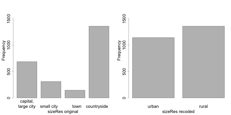
Fig. 4 Effect of recoding – frequency counts before and after recoding

Global recoding of a numerical (continuous) variables changes it into a categorical variable. The intervals should cover the entire value range of the variable. Fig. 5 shows the effect of recoding the variable “age”, age in years, in ten-year intervals.

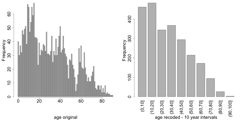
Fig. 5 Age variable before and after recoding

Instead of creating intervals of equal width, we can also create intervals of unequal width. This is illustrated in code53, where we use the age groups 1-5, 6-11, 12-17, 18-21, 22-25, 26-49, 50-64 and 65+. In this example, this is a useful step, since even after recoding in 10-year intervals, the categories with high age values have low frequencies. We chose the intervals by respecting relevant school age and employment age values (e.g., retirement age is 65 in this example) such that the data can still be used for common research on education and employment. Fig. 6 shows the effect of recoding the variable “age” after adjusting the intervals.

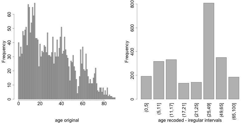
Fig. 6 Age variable before and after recoding

Top and bottom coding¶

Top and bottom coding are similar to global recoding, but instead of recoding all values, only the top and/or bottom values of the distribution or categories are recoded. This can be applied only to ordinal categorical variables and (semi-)continuous variables, since the values have to be at least ordered. Top and bottom coding is especially useful if the bulk of the values lies in the center of the distribution with the peripheral categories having only few observations (outliers). Examples are age and income; for these variables, there will often be only a few observations above certain thresholds, typically at the tails of the distribution. The fewer the observations within a category, the higher the identification risk. One solution could be grouping the values at the tails of the distribution into one category. This reduces the risk for those observations, and, importantly, does so without reducing the data utility for the other observations in the distribution.

Deciding where to apply the threshold and what observations should be grouped requires:

Reviewing the overall distribution of the variable to identify at which point the frequencies drop below the desired number of observations and identify outliers in the distribution. Fig. 7 shows the distribution of the age variable and suggests 65 (red vertical line) for the top code age.
Taking into account the intended use of the data and the purpose for which the survey was conducted. For example, if the data are typically used to measure labor force participation for those aged 15 to 64, then top and bottom coding should not interfere with the categories 15 to 64. Otherwise the analyst would find it impossible to create the desired measures for which the data were intended. In the example, we consider this and code all age higher than 64.

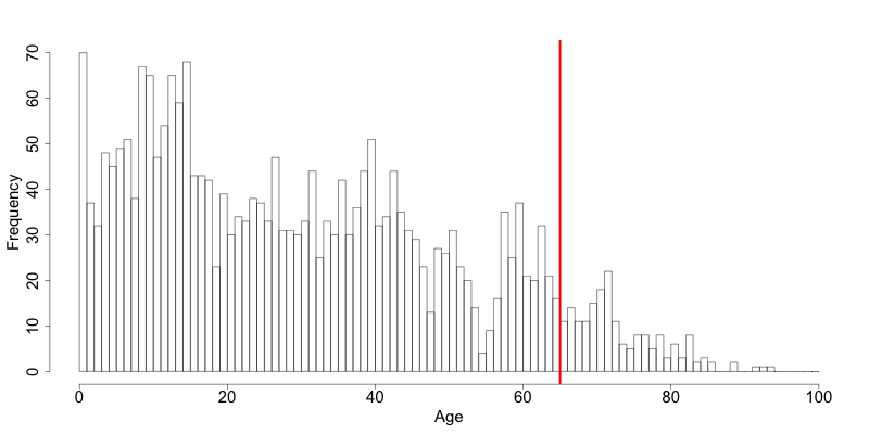
Fig. 7 Utilizing the frequency distribution of variable age to determine threshold for top coding

Rounding¶

Rounding is similar to grouping, but used for continuous variables. Rounding is useful to prevent exact matching with external data sources. In addition, it can be used to reduce the level of detail in the data. Examples are removing decimal figures or rounding to the nearest 1,000.

The next section discusses the method local suppression. Recoding is often used before local suppression to reduce the number of necessary suppressions.

Recommended Reading Material on Recoding

Hundepool, Anco, Josep Domingo-Ferrer, Luisa Franconi, Sarah Giessing, Rainer Lenz, Jane Naylor, Eric Schulte Nordholt, Giovanni Seri, and Peter Paul de Wolf. 2006. Handbook on Statistical Disclosure Control. ESSNet SDC. http://neon.vb.cbs.nl/casc/handbook.htm.

Hundepool, Anco, Josep Domingo-Ferrer, Luisa Franconi, Sarah Giessing, Eric Schulte Nordholt, Keith Spicer, and Peter Paul de Wolf. 2012. Statistical Disclosure Control. Chichester: John Wiley & Sons Ltd. doi:10.1002/9781118348239.

Templ, Matthias, Bernhard Meindl, Alexander Kowarik, and Shuang Chen. 2014. Statistical Disclosure Control (SDCMicro). http://www.ihsn.org/home/software/disclosure-control-toolbox. (accessed June 9, 2018).

De Waal, A.G., and Willenborg, L.C.R.J. 1999. Information loss through global recoding and local suppression. Netherlands Official Statistics, 14:17-20, 1999. Special issue on SDC

Local suppression¶

It is common in surveys to encounter values for certain variables or combinations of quasi-identifiers (keys) that are shared by very few individuals. When this occurs, the risk of re-identification for those respondents is higher than the rest of the respondents (see the Section k-anonymity). Often local suppression is used after reducing the number of keys in the data by recoding the appropriate variables. Recoding reduces the number of necessary suppressions as well as the computation time needed for suppression. Suppression of values means that values of a variable are replaced by a missing value. The Section k-anonymity discusses how missing values influence frequency counts and \(k\)-anonymity. It is important to note that not all values for all individuals of a certain variable are suppressed, which would be the case when removing a direct identifier, such as “name”; only certain values for a particular variable and a particular respondent or set of respondents are suppressed. This is illustrated in the following example and Table 9.

Table 9 presents a dataset with seven respondents and three quasi-identifiers. The combination {‘female’, ‘rural’, ‘higher’} for the variables “gender”, “region” and “education” is an unsafe combination, since it is unique in the sample. By suppressing either the value ‘female’ or ‘higher’, the respondent cannot be distinguished from the other respondents anymore, since that respondent shares the same combination of key variables with at least three other respondents. Only the value in the unsafe combination of the single respondent at risk is suppressed, not the values for the same variable of the other respondents. The freedom to choose which value to suppress can be used to minimize the total number of suppressions and hence the information loss. In addition, if one variable is very important to the user, we can choose not to suppress values of this variable, unless strictly necessary. In the example, we can choose between suppressing the value ‘female’ or ‘higher’ to achieve a safe data file; we chose to suppress ‘higher’. This choice should be made taking into account the needs of data users. In this example we find “gender” more important than “education”.

Table 9 Local suppression illustration - sample data before and after suppression¶
Variable	Before local suppression			After local suppression
ID	Gender	Region	Education	Gender	Region	Education
1	female	rural	higher	female	rural	missing
2	male	rural	higher	male	rural	higher
3	male	rural	higher	male	rural	higher
4	male	rural	higher	male	rural	higher
5	female	rural	lower	female	rural	lower
6	female	rural	lower	female	rural	lower
7	female	rural	lower	female	rural	lower

Since continuous variables have a high number of unique values (e.g., income in dollars or age in years), \(k\)-anonymity and local suppression are not suitable for continuous variables or variables with a very high number of categories. A possible solution in those cases might be to first recode to produce fewer categories (e.g., recoding age in 10-year intervals or income in quintiles). Always keep in mind, though, what effect any recoding will have on the utility of the data.

Several different algorithms can be used to determine which values to suppress. One common algorithm determines an optimal suppression pattern to achieve on a specified set of quasi-identifiers a certain level of \(k\)-anonymity for these quasi-identifiers. This algorithm used seeks to minimize the total number of suppressions while achieving the required \(k\)-anonymity threshold. By default, this algorithm is more likely to suppress values of variables with many different categories or values, and less likely to suppress variables with fewer categories. For example, the values of a geographical variable, with 12 different areas, are more likely to be suppressed than the values of the variable “gender”, which has typically only two categories. If variables with many different values are important for data utility and suppression is not desired for them, one can rank variables by importance and thus specify the order in which the algorithm will seek to suppress values within quasi-identifiers to achieve \(k\)-anonymity. The algorithm seeks to apply fewer suppressions to variables of high importance than to variables with lower importance. Nevertheless, suppressions in the variables with high importance might be inevitable to achieve the required level of \(k\)-anonymity.

Example of local suppression¶

In this example local suppression is applied to achieve the \(k\)-anonymity threshold of 5 on the quasi-identifiers “gender”, “region”, “religion”, “age” and “ethnicity”. Without ranking the importance of the variables, the value of the variable “age” is more likely to be suppressed, since this is the variable with most categories. The variable “age” has 10 categories after recoding. The variable “gender” is least likely to be suppressed, since it has only two different values: ‘male’ and ‘female’. The other variables have 4 (“sizeRes”), 2 (“region”), and 8 (“ethnicity”) categories. The standard local suppression algorithm suppresses most values in the variable “age” (80). In fact, only the variable “ethnicity” of the other variables also needed suppressions (8) to achieve the \(k\)-anonymity threshold of 5. The variable “ethnicity” is the variable with the second highest number of suppressions.

The variable “age” is typically an important variable. Therefore, if possible, we would like to reduce the number of suppressions on “age” by specifying the order of importance of the variables and giving high importance (little suppression) to the quasi-identifier “age”. We also assign importance to the variable “gender”. The effect is clear: there are no suppressions in the variables “age” and “gender”. For that, the other variables, especially “sizeRes” (87) and “ethnicity” (62), received many more suppressions. The total number of suppressed values has increased from 88 to 166.

Note

Fewer suppressions in one variable increase the number of necessary suppressions in other variables.

Generally, the total number of suppressed values needed to achieve the required level of \(k\)-anonymity increases when specifying the order of importance, since this prevents to use the optimal suppression pattern. The importance of variables should be specified only in cases where the variables with many categories play an important role in data utility for the data users [1].

Fig. 8 demonstrates the effect of the required \(k\)-anonymity threshold and the order of importance on the data utility by using several labor market-related indicators from an I2D2 [2] dataset before and after anonymization. Fig. 8 displays the relative changes as a percentage of the initial value after re-computing the indicators with the data to which local suppression was applied. The indicators are the proportion of active females and males, and the number of females and males of working age. The values computed from the raw data were, respectively, 68%, 12%, 8,943 and 9,702. The vertical line at 0 is the benchmark of no change. The numbers indicate the required k-anonymity threshold (3 or 5) and the colors indicate the importance vector: red (no symbol) is no importance vector, blue (with * symbol) is high importance on the variable with the employment status information and dark green (with + symbol) is high importance on the age variable.

A higher \(k\)-anonymity threshold leads to greater information loss (i.e., larger deviations from the original values of the indicators, the 5’s are further away from the benchmark of no change than the corresponding 3’s) caused by local suppression. Reducing the number of suppressions on the employment status variable by specifying an importance vector does not improve the indicators. Instead, reducing the number of suppressions on age greatly reduces the information loss. Since specific age groups have a large influence on the computation of these indicators (the rare cases are in the extremes and will be suppressed), high suppression rates on age distort the indicators. It is generally useful to compare utility measures (see the Section Measuring Utility and Information Loss ) to specify the importance vector, since the effects can be unpredictable.

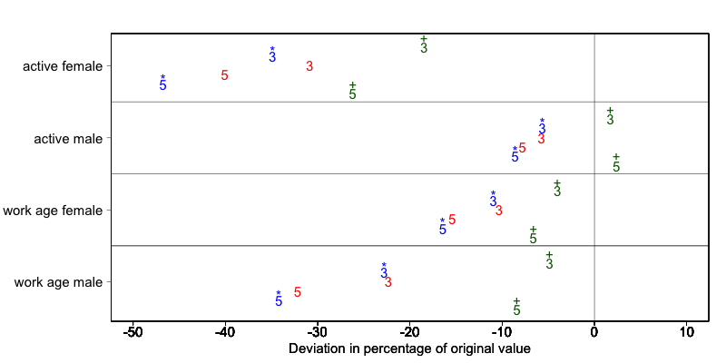
Fig. 8 Changes in labor market indicators after anonymization of I2D2 data

The threshold of \(k\)-anonymity to be set depends on several factors, which are amongst others: 1) the legal requirements for a safe data file; 2) other methods that will be applied to the data; 3) the number of suppressions and related information loss resulting from higher thresholds; 4) the type of variable; 5) the sample weights and sample size; and 6) the release type (see the Section Release Types ). Commonly applied levels for the \(k\)-anonymity threshold are 3 and 5.

Table 10 illustrates the influence of specifying the order of importance and the \(k\)-anonymity threshold on the global risk after suppression and total number of suppressions required to achieve this \(k\)-anonymity threshold. The dataset contains about 63,000 individuals. The higher the \(k\)-anonymity threshold, the more suppressions are needed and the lower the risk after local suppression (expected number of re-identifications). In this particular example, the computation time is shorter for higher thresholds. This is due the higher number of necessary suppressions, which reduces the difficulty of the search for an optimal suppression pattern.

The age variable is recoded in five-year intervals and has 20 age categories. This is the variable with the highest number of categories. Prioritizing the suppression of other variables leads to a higher total number of suppressions and a longer computation time.

Table 10 How the order of importance and the \(k\)-anonymity threshold affect total number of suppressions¶
Threshold	Importance	Total number of	Threshold	Total number of
k-anonimity	vector	suppressions	k-anonimity	suppressions
3	none (default)	6,676	5,387	11.8
3	employment status	7,254	5,512	13.1
3	age variable	8,175	60	4.5
5	none (default)	9,971	7,894	8.5
5	employment status	11,668	8,469	10.2
5	age variable	13,368	58	3.8

In cases where there are a large number of quasi-identifiers and the variables have many categories, the number of possible combinations increases rapidly (see \(k\)-anonymity). If the number of variables and categories is very large, the computation time of the local suppression algorithms can be very long. Therefore, reducing the number of quasi-identifiers and/or categories before applying local suppression is recommended. This can be done by recoding variables or selecting some variables for other (perturbative) methods, such as PRAM. This is to ensure that the number of suppressions is limited and hence the loss of data is limited to only those values that pose most risk.

All-m approach¶

In some datasets, it might prove difficult to reduce the number of quasi-identifiers and even after reducing the number of categories by recoding, the local suppression algorithm takes a long time to compute the required suppressions. A solution in such cases can be the so-called ‘all-\(m\) approach’ (see Wolf15). The all-\(m\) approach consists of applying the local suppression algorithm as described above to all possible subsets of size \(m\) of the total set of quasi-identifiers. The advantage of this approach is that the partial problems are easier to solve and computation time will be slower. Caution should be applied since this method does not necessarily lead to \(k\)-anonymity in the complete set of quasi-identifiers. There are two possibilities to reach the same level of protection: 1) to choose a higher threshold for \(k\) or 2) to re-apply the local suppression algorithm on the complete set of quasi-identifiers after using the all-\(m\) approach to achieve the required threshold. In the second case, the all-\(m\) approach leads to a shorter computation time at the cost of a higher total number of suppressions.

Note

The required level is not achieved automatically on the entire set of quasi-identifiers if the all-m approach is used.

Therefore, it is important to evaluate the risk measures carefully after using the all-\(m\) approach.

Table 11 presents the results of using the all-\(m\) approach of a test dataset with 9 key variables and 4,000 records. The table shows the parameters ’k’ and ‘combs’, which are respectively the \(k\)-anonymity threshold and the size of the subsets, the number of \(k\)-anonymity violators for different levels of \(k\) as well as the total number of suppressions. We observe that the different combinations do not always lead to the required level of \(k\)-anonimity. For example, when setting \(k = 3\), and combs 3 and 7, there are still 15 records in the dataset (with a total of 9 quasi-identifiers) that violate 3-anonimity after local suppression. Due to the smaller sample size, the gains in running time are not yet apparent in this example, since the rerunning algorithm several times takes up time. A larger dataset would benefit more from the all-\(m\) approach, as the algorithm would take longer in the first place.

Table 11 Effect of the all-\(m\) approach on k-anonymity¶
Arguments		Number of violators for different levels of \(k\)-anonimity on complete set			Total number of suppressions
k	combs	k = 2	k = 3	k = 5
Before local suppression		2,464	3,324	3,877	0
3	.	0	0	1,766	2,264
5	.	0	0	0	3,318
3	3	2,226	3,202	3,819	3,873
3	3, 7	15	108	1,831	6,164
3	3, 9	0	0	1,794	5,982
3	5, 9	0	0	1,734	6,144
5	3	2,047	3,043	3,769	3,966
5	3, 7	0	6	86	7,112
5	3, 9	0	0	0	7,049
5	5, 9	0	0	0	7,129
5, 3	3, 7	11	108	1,859	6,140
5, 3	3, 9	0	0	1,766	2,264
5, 3	5, 9	0	0	0	3,318

Often the dataset contains variables that are related to the key variables used for local suppression. Examples are rural/urban to regions in case regions are completely rural or urban or variables that are only answered for specific categories (e.g., sector for those working, schooling related variables for certain age ranges). In those cases, the variables rural/urban or sector might not be quasi-identifiers themselves, but could allow the intruder to reconstruct suppressed values in the quasi-identifiers region or employment status. For example, if region 1 is completely urban, and all other regions are only semi-urban or rural, a suppression in the variable region for a record in region 1 can be simply reconstructed by the rural/urban variable. Therefore, it is useful to suppress the values corresponding to the suppressions in those linked variables.

Another simpler alternative for the local suppression algorithm described above is to suppress values of certain key variables of individuals with risks above a certain threshold. In this case, all values of the specified variable for respondents with a risk higher than the specified threshold will be suppressed. The risk measure used is the individual risk (see the Section Individual risk). This is useful if one variable has sensitive values that should not be released for individuals with high risks of re-identification. What is considered high re-identification probability depends on legal requirements.

Perturbative methods¶

Perturbative methods do not suppress values in the dataset, but perturb (alter) values to limit disclosure risk by creating uncertainty around the true values. An intruder is uncertain whether a match between the microdata and an external file is correct or not. Most perturbative methods are based on the principle of matrix masking, i.e., the altered dataset \(Z\) is computed as

\[Z = AXB + C\]

where \(X\) is the original data, \(A\) is a matrix used to transform the records, \(B\) is a matrix to transform the variables and \(C\) is a matrix with additive noise.

Note

Risk measures based on frequency counts of keys are no longer valid after applying perturbative methods.

This can be seen in Table 12 , which displays the same data before and after swapping some values. The swapped values are in italics. Both before and after perturbing the data, all observations violate \(k\)-anonymity at the level 3 (i.e., each key does not appear more than twice in the dataset). Nevertheless, the risk of correct re-identification of the records is reduced and hence information contained in other (sensitive) variables possibly not disclosed. With a certain probability, a match of the microdata with an external data file will be wrong. For example, an intruder would find one individual with the combination {‘male’, ‘urban’, ‘higher’}, which is a sample unique. However, this match is not correct, since the original dataset did not contain any individual with these characteristics and hence the matched individual cannot be a correct match. The intruder cannot know with certainty whether the information disclosed from other variables for that record is correct.

Table 12 Sample data before and after perturbation¶
Variable	Original data			After perturbing the data
ID	Gender	Region	Education	Gender	Region	Education
1	female	rural	higher	female	rural	higher
2	female	rural	higher	female	rural	lower
3	male	rural	lower	male	rural	lower
4	male	rural	lower	female	rural	lower
5	female	urban	lower	male	urban	higher
6	female	urban	lower	female	urban	lower

One advantage of perturbative methods is that the information loss is reduced, since no values will be suppressed, depending on the level of perturbation. One disadvantage is that data users might have the impression that the data was not anonymized before release and will be less willing to participate in future surveys. Therefore, there is a need for reporting both for internal and external use (see the Section Step 11: Audit and Reporting).

An alternative to perturbative methods is the generation of synthetic data files with the same characteristics as the original data files. Synthetic data files are not discussed in these guidelines. For more information and an overview of the use of synthetic data as SDC method, we refer to Drec11 and Section 3.8 in HDFG12. We discuss here five perturbative methods: Post Randomization Method (PRAM), microaggregation, noise addition, shuffling and rank swapping.

PRAM (Post RAndomization Method)¶

PRAM is a perturbative method for categorical data. This method reclassifies the values of one or more variables, such that intruders that attempt to re-identify individuals in the data do so, but with positive probability, the re-identification made is with the wrong individual. This means that the intruder might be able to match several individuals between external files and the released data files, but cannot be sure whether these matches are to the correct individual.

PRAM is defined by the transition matrix \(P\), which specifies the transition probabilities, i.e., the probability that a value of a certain variable stays unchanged or is changed to any of the other \(k - 1\) values. \(k\) is the number of categories or factor levels within the variable to be PRAMmed. For example, if the variable region has 10 different regions, \(k\) equals 10. In case of PRAM for a single variable, the transition matrix is size \(k*k\). We illustrate PRAM with an example of the variable “region”, which has three different values: ‘capital’, ‘rural1’ and ‘rural2’. The transition matrix for applying PRAM to this variable is size 3*3:

\[\begin{split}P = \begin{bmatrix} 1 & 0 & 0 \\ 0.05 & 0.8 & 0.15 \\ 0.05 & 0.15 & 0.8 \\ \end{bmatrix}\end{split}\]

The values on the diagonal are the probabilities that a value in the corresponding category is not changed. The value 1 at position (1,1) in the matrix means that all values ‘capital’ stay ‘capital’; this might be a useful decision, since most individuals live in the capital and no protection is needed. The value 0.8 at position (2,2) means that an individual with value ‘rural1’ will stay with probability 0.8 ‘rural1’. The values 0.05 and 0.15 in the second row of the matrix indicate that the value ‘rural1’ will be changed to ‘capital’ or ‘rural2’ with respectively probability 0.05 and 0.15. If in the initial file we had 5,000 individuals with value ‘capital’ and resp. 500 and 400 with values ‘rural1’ and ‘rural2’, we expect after applying PRAM to have 5,045 individuals with capital, 460 with rural1 and 395 with rural2 [3]. The recoding is done independently for each individual. We see that the tabulation of the variable “region” yields different results before and after PRAM, which are shown in Table 13. The deviation from the expectation is due to the fact that PRAM is a probabilistic method, i.e., the results depend on a probability-generating mechanism; consequently, the results can differ every time we apply PRAM to the same variables of a dataset.

Note

The number of changed values is larger than one might think when inspecting the tabulations in Table 13. Not all 5,052 individuals with value capital after PRAM had this value before PRAM and the 457 individuals in rural1 after PRAM are not all included in the 500 individuals before PRAM. The number of changes is larger than the differences in the tabulation (cf. transition matrix).

Given that the transition matrix is known to the end users, there are several ways to correct statistical analysis of the data for the distortions introduced by PRAM.

Table 13 Tabulation of variable “region” before and after PRAM¶
Value	Tabulation before PRAM	Tabulation after PRAM
capital	5,000	5,052
rural1	500	457
rural2	400	391

One way to guarantee consistency between the tabulations before and after PRAM is to choose the transition matrix so that, in expectation, the tabulations before and after applying PRAM are the same for all variables. This condition is fulfilled if the vector with the tabulation of the absolute frequencies of the different categories in the original data is an eigenvector of the transition matrix that corresponds to the unit eigenvalue. PRAM using such transition matrix is called invariant PRAM.

Note

Invariant does not guarantee that cross-tabulations of variables (unlike univariate tabulations) stay the same.

PRAM is a probabilistic method and the results can differ every time we apply PRAM to the same variables of a dataset. To overcome this and make the results reproducible, it is good practice to set a seed for the random number generator, so the same random numbers will be generated every time.

Table 14 shows the tabulation of the variable after applying invariant PRAM. We can see that the deviations from the initial tabulations, which are in expectation 0, are smaller than with the transition matrix that does not fulfill the invariance property. The remaining deviations are due to the randomness.

Table 14 Tabulation of variable “region” before and after (invariant) PRAM¶
Value	Tabulation before PRAM	Tabulation after PRAM	Tabulation after invariant PRAM
capital	5,000	5,052	4,998
rural1	500	457	499
rural2	400	391	403

Table 15 presents the cross-tabulations with the variable gender. Before applying invariant PRAM, the share of males in the city is much higher than the share of females (about 60%). This property is not maintained after invariant PRAM (the shares of males and females in the city are roughly equal), although the univariate tabulations are maintained. One solution is to apply PRAM separately for the males and females in this example [4].

Table 15 Cross-tabulation of variable “region” and variable “gender” before and after invariant PRAM¶
.	Tabulation before PRAM		Tabulation after invariant PRAM
Value	male	female	male	female
capital	3,056	1,944	2,623	2,375
rural1	157	343	225	274
rural2	113	287	187	216

PRAM is especially useful when a dataset contains many variables and applying other anonymization methods, such as recoding and local suppression, would lead to significant information loss. Checks on risk and utility are important after PRAM.

To do statistical inference on variables to which PRAM was applied, the researcher needs knowledge about the PRAM method as well as about the transition matrix. The transition matrix, together with the random number seed, can, however, lead to disclosure through reconstruction of the non-perturbed values. Therefore, publishing the transition matrix but not the random seed is recommended.

A disadvantage of using PRAM is that very unlikely combinations can be generated, such as a 63-year-old who goes to school. Therefore, the PRAMmed variables need to be audited to prevent such combinations from happening in the released data file. In principal, the transition matrix can be designed in such a way that certain transitions are not possible (probability 0). For instance, for those that go to school, the age must range within 6 to 18 years and only such changes are allowed.

This is illustrated in the following example. Assume, we have two variables “toilet” and “region” and the variable “toilet” needs to be PRAMmed. By applying PRAM to the variable “toilet” within the strata generated by the “region” variable, we prevent changes in the variable “toilet”, where toilet types in a particular region are exchanged with those in other regions. For instance, in the capital region certain types of unimproved toilet types are not in use and therefore these combinations should not occur after PRAMming. Values are only changed with those that are available in the same strata. Strata can be formed by any categorical variable, e.g., gender, age groups, education level.

Microaggregation¶

Microaggregation is most suitable for continuous variables, but can be extended in some cases to categorical variables. [5] It is most useful where confidentiality rules have been predetermined (e.g., a certain threshold for \(k\)-anonymity has been set) that permit the release of data only if combinations of variables are shared by more than a predetermined threshold number of respondents (\(k\)). The first step in microaggregation is the formation of small groups of individuals that are homogeneous with respect to the values of selected variables, such as groups with similar income or age. Subsequently, the values of the selected variables of all group members are replaced with a common value, e.g., the mean of that group. Microaggregation methods differ with respect to (i) how the homogeneity of groups is defined, (ii) the algorithms used to find homogeneous groups, and (iii) the determination of replacement values. In practice, microaggregation works best when the values of the variables in the groups are more homogeneous. When this is the case, then the information loss due to replacing values with common values for the group will be smaller than in cases where groups are less homogeneous.

In the univariate case, and also for ordinal categorical variables, formation of homogeneous groups is straightforward: groups are formed by first ordering the values of the variable and then creating \(g\) groups of size \(n_{i}\) for all groups \(i\) in \(1,\ \ldots,\ g\). This maximizes the within-group homogeneity, which is measured by the within-groups sum of squares (\(SSE\))

\[SSE = \sum_{i = 1}^{g}{\sum_{j = 1}^{n_{i}}{\left( x_{ij} - {\overline{x}}_{i} \right)^{T}\left( x_{ij} - {\overline{x}}_{i} \right)}}\]

The lower the SSE, the higher the within-group homogeneity. The group sizes can differ amongst groups, but often groups of equal size are used to simplify the search [6].

Choice of group size depends on the homogeneity within the groups and the required level of protection. In general it holds that the larger the group, the higher the protection. A disadvantage of groups of equal sizes is that the data might be unsuitable for this. For instance, if two individuals have a low income (e.g., 832 and 966) and four individuals have a high income (e.g., 3,313, 3,211, 2,987, 3,088), the mean of two groups of size three (e.g., (832 + 966 + 2,987) / 3 = 1,595 and (3,088 + 3,211 + 3,313) / 3 = 3,204) would represent neither the low nor the high income.

Often, values are replaced by the group mean. An alternative, more robust approach is to replace group values with the median. In cases where the median is chosen, one individual in every group keeps the same value if groups have odd sizes. In cases where there is a high degree of heterogeneity within the groups (this is often the case for larger groups), the median is preferred to preserve the information in the data. An example is income, where one outlier can lead to multiple outliers being created when using microaggregation. This is illustrated in Table 16. If we choose the mean as replacement for all values, which are grouped with the outlier (6,045 in group 2), these records will be assigned values far from their original values. If we chose the median, the incomes of individuals 1 and 2 are not perturbed, but no value is an outlier. Of course, this might in itself present problems.

Note

If microaggregation alters outlying values, this can have a significant impact on the computation of some measures sensitive to outliers, such as the GINI index.

In the case where microaggregation is applied to categorical variables, the median is used to calculate the replacement value for the group.

Table 16 Illustrating the effect of choosing mean vs. median for microaggregation where outliers are concerned¶
ID	Group	Income	Microaggregation (mean)	Microaggregation (median)
1	1	2,300	2,245	2,300
2	2	2,434	3,608	2,434
3	1	2,123	2,245	2,300
4	1	2,312	2,245	2,300
5	2	6,045	3,608	2,434
6	2	2,345	3,608	2,434

In case of multiple variables that are candidates for microaggregation, one possibility is to apply univariate microaggregation to each of the variables separately. The advantage of univariate microaggregation is minimal information loss, since the changes in the variables are limited. The literature shows, however, that disclosure risk can be very high if univariate microaggregation is applied to several variables separately and no additional anonymization techniques are applied (DMOT02). To overcome this shortcoming, an alternative to univariate microaggregation is multivariate microaggregation.

Multivariate microaggregation is widely used in official statistics. The first step in multivariate aggregation is the creation of homogeneous groups based on several variables. Groups are formed based on multivariate distances between the individuals. Subsequently, the values of all variables for all group members are replaced with the same values. Table 17 illustrates this with three variables. We see that the grouping by income, expenditure and wealth leads to a different grouping, as in the case in Table 16, where groups were formed based only on income.

Table 17 Illustration of multivariate microaggregation¶
ID	Group	Before microaggregation			After microaggregation
.	.	Income	Exp	Wealth	Income	Exp	Wealth
1	1	2,300	1,714	5.3	2,285.7	1,846.3	6.3
2	1	2,434	1,947	7.4	2,285.7	1,846.3	6.3
3	1	2,123	1,878	6.3	2,285.7	1,846.3	6.3
4	2	2,312	1,950	8.0	3,567.3	2,814.0	8.3
5	2	6,045	4,569	9.2	3,567.3	2,814.0	8.3
6	2	2,345	1,923	7.8	3,567.3	2,814.0	8.3

There are several multivariate microaggregation methods that differ with respect to the algorithm used for creating groups of individuals. There is a trade-off between speed of the algorithm and within-group homogeneity, which is directly related to information loss. For large datasets, this is especially challenging. We discuss the Maximum Distance to Average Vector (MDAV) algorithm here in more detail. The MDAV algorithm was first introduced by DoTo05 and represents a good choice with respect to the trade-off between computation time and the group homogeneity, computed by the within-group \(SSE\).

The algorithm computes an average record or centroid C, which contains the average values of all included variables. We select an individual A with the largest squared Euclidean distance from C, and build a group of \(k\) records around A. The group of \(k\) records is made up of A and the \(k-1\) records closest to A measured by the Euclidean distance. Next, we select another individual B, with the largest squared Euclidean distance from individual A. With the remaining records, we build a group of \(k\) records around B. In the same manner, we select an individual D with the largest distance from B and, with the remaining records, build a new group of \(k\) records around D. The process is repeated until we have fewer than \(2*k\) records remaining. The MDAV algorithm creates groups of equal size with the exception of maybe one last group of remainders. The microaggregated dataset is then computed by replacing each record in the original dataset by the average values of the group to which it belongs. Equal group sizes, however, may not be ideal for data characterized by greater variability. The MDAV algorithm is illustrated in Fig. 9.

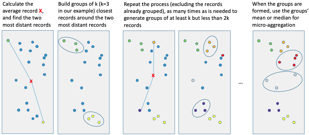
Fig. 9 Illustration of MDAV algorithm

It is also possible to group variables only within strata. This reduces the computation time and adds an extra layer of protection to the data, because of the greater uncertainty produced [7].

Besides the method MDAV, there are few other grouping methods implemented in standard SDC software, such as sdcMicro (TeMK14). The differences are mainly the distance measure (Euclidean distance, Mahalanobis distance) or sorting based on the first principal component and whether clustering is used. The first principal component (PC) is the projection of all variables into a one-dimensional space maximizing the variance of this projection. The performance of this method depends on the share of the total variance in the data that is explained by the first PC. Using the Mahalanobis distance is computationally more intensive, but provides better results with respect to group homogeneity. It is recommended for smaller datasets (TeMK14).

In case of several variables to be used for microaggregation, looking first at the covariance or correlation matrix of these variables is recommended. If not all variables correlate well, but two or more sets of variables show high correlation, less information loss will occur when applying microaggregation separately to these sets of variables. In general, less information loss will occur when applying multivariate microaggregation, if the variables are highly correlated. The advantage of replacing the values with the mean of the groups rather than other replacement values has the advantage that the overall means of the variables are preserved.

Recommended Reading Material on Microaggregation

Domingo-Ferrer, Josep, and Josep Maria Mateo-Sanz. 2002.”Practical data-oriented microaggregation for statistical disclosure control.” IEEE Transactions on Knowledge and Data Engineering 14 (2002): 189-201.

Hansen, Stephen Lee, and Sumitra Mukherjee. 2003. “A polynomial algorithm for univariate optimal.” IEEE Transactions on Knowledge and Data Engineering 15 (2003): 1043-1044.

Hundepool, Anco, Josep Domingo-Ferrer, Luisa Franconi, Sarah Giessing, Rainer Lenz, Jane Naylor, Eric Schulte Nordholt, Giovanni Seri, and Peter Paul de Wolf. 2006. Handbook on Statistical Disclosure Control. ESSNet SDC. http://neon.vb.cbs.nl/casc/handbook.htm

Hundepool, Anco, Josep Domingo-Ferrer, Luisa Franconi, Sarah Giessing, Eric Schulte Nordholt, Keith Spicer, and Peter Paul de Wolf. 2012. Statistical Disclosure Control. Chichester: John Wiley & Sons Ltd. doi:10.1002/9781118348239.

Templ, Matthias, Bernhard Meindl, Alexander Kowarik, and Shuang Chen. 2014, August. “International Household Survey Network (IHSN).” http://www.ihsn.org/home/software/disclosure-control-toolbox. (accessed July 9, 2018).

Noise addition¶

Noise addition, or noise masking, means adding or subtracting (small) values to the original values of a variable, and is most suited to protect continuous variables (see Bran02 for an overview). Noise addition can prevent exact matching of continuous variables. The advantages of noise addition are that the noise is typically continuous with mean zero, and exact matching with external files will not be possible. Depending on the magnitude of noise added, however, approximate interval matching might still be possible.

When using noise addition to protect data, it is important to consider the type of data, the intended use of the data and the properties of the data before and after noise addition, i.e., the distribution – particularly the mean – covariance and correlation between the perturbed and original datasets.

Depending on the data, it may also be useful to check that the perturbed values fall within a meaningful range of values. Fig. 11 illustrates the changes in data distribution with increasing levels of noise. For data that has outliers, it is important to note that when the perturbed data distribution is similar to the original data distribution (e.g., at low noise levels), noise addition will not protect outliers. After noise addition, these outliers can generally still be detected as outliers and hence easily be identified. An example is a single very high income in a certain region. After perturbing this income value, the value will still be recognized as the highest income in that region and can thus be used for re-identification. This is illustrated in Fig. 10, where 10 original observations (open circles) and the anonymized observations (red triangles) are plotted. The tenth observation is an outlier. The values of the first nine observations are sufficiently protected by adding noise: their magnitude and order has changed and exact or interval matching can be successfully prevented. The outlier is not sufficiently protected since, after noise addition, the outlier can still be easily identified. The fact that the absolute value has changed is not sufficient protection. On the other hand, at high noise levels, protection is higher even for the outliers, but the data structure is not preserved and the information loss is large, which is not an ideal situation. One way to circumvent the outlier problem is to add noise of larger magnitude to outliers than to the other values.

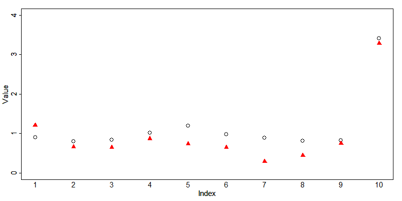
Fig. 10 Illustration of effect of noise addition to outliers

There are several noise addition algorithms. The simplest version of noise addition is uncorrelated additive normally distributed noise, where \(x_{j}\), the original values of variable \(j\)are replaced by

\[z_{j} = x_{j} + \varepsilon_{j},\]

where \(\varepsilon_{j}\ \sim\ N(0,\ \ \sigma_{\varepsilon_{j}}^{2})\ \)and \(\sigma_{\varepsilon_{j}} = \alpha * \sigma_{j}\) with \(\sigma_{j}\) the standard deviation of the original data. In this way, the mean and the covariances are preserved, but not the variances and correlation coefficient. If the level of noise added, \(\alpha\), is disclosed to the user, many statistics can be consistently estimated from the perturbed data. The added noise is proportional to the variance of the original variable. The magnitude of the noise added is specified by the parameter \(\alpha\), which specifies this proportion. The standard deviation of the perturbed data is \(1 + \alpha\) times the standard deviation of the perturbed data. A decision on the magnitude of noise added should be informed by the legal situation regarding data privacy, data sensitivity and the acceptable levels of disclosure risk and information loss. In general, the level of noise is a function of the variance of the original variables, the level of protection needed and the desired value range after anonymization [8]. An \(\alpha\) value that is too small will lead to insufficient protection, while an \(\alpha\) value that is too high will make the data useless for data users.

Fig. 11 shows the frequency distribution of a numeric continuous variable and the distribution before and after noise addition with different levels of noise (0.1, 0.5, 1, 2 and 5). The first plot shows the distribution of the original values. The histograms clearly show that noise of large magnitudes (high values of alpha) lead to a distribution of the data far from the original values. The distribution of the data changes to a normal distribution when the magnitude of the noise grows respective to the variance of the data. The mean in the data is preserved, but, with an increased level of noise, the variance of the perturbed data grows. After adding noise of magnitude 5, the distribution of the original data is completely destroyed.

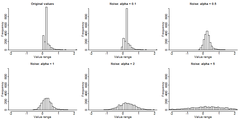
Fig. 11 Frequency distribution of a continuous variable before and after noise addition

Fig. 12 shows the value range of a variable before adding noise (no noise) and after adding several levels of noise (\(\alpha\) from 0.1 to 1.5 with 0.1 increments). In the figure, the minimum value, the 20^th, 30^th, 40^th percentiles, the median, the 60^th, 70^th, 80^th and 90^th percentiles and the maximum value are plotted. The median (50^th percentile) is indicated with the red “+” symbol. From Fig. 11 and Fig. 12, it is apparent that the range of values expands after noise addition, and the median stays roughly at the same level, as does the mean by construction. The larger the magnitude of noise added, the wider the value range. In cases where the variable should stay in a certain value range (e.g., only positive values, between 0 and 100), this can be a disadvantage of noise addition. For instance, expenditure variables typically have non-negative values, but adding noise to these variables can generate negative values, which are difficult to interpret. One way to get around this problem is to set any negative values to zero. This truncation of values below a certain threshold, however, will distort the distribution (mean and variance matrix) of the perturbed data. This means that the characteristics that were preserved by noise addition, such as the conservation of the mean and covariance matrix, are destroyed and the user, even with knowledge of the magnitude of the noise, can no longer use the data for consistent estimation.

Another way to avoid negative values is the application of multiplicative rather than additive noise. In that case, variables are multiplied by a random factor with expectation 1 and a positive variance. This will also lead to larger perturbations (in absolute value) of large initial values (outliers). If the variance of the noise added is small, there will be no or few negative factors and thus fewer sign changes than in case of additive noise masking. Multiplicative noise masking is not implemented in sdcMicro, but can be relatively easily implemented in base R by generating a vector of random numbers and multiplying the data with this vector. For more information on multiplicative noise masking and the properties of the data after masking, we refer to KiWi03.

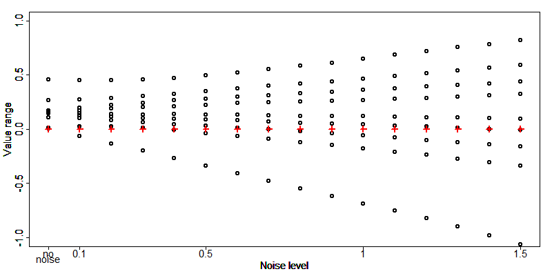
Fig. 12 Noise levels and the impact on the value range (percentiles)

If two or more variables are selected for noise addition, correlated noise addition is preferred to preserve the correlation structure in the data. In this case, the covariance matrix of noise \(\Sigma_{\varepsilon}\ \)is proportional to the covariance matrix of the original data \(\Sigma_{X}:\)

\[\Sigma_{\varepsilon} = \alpha \Sigma_{X}\]

If noise addition is applied to variables that are a ratio of an aggregate, this structure can be destroyed by noise addition. Examples are income and expenditure data with many income and expenditure categories. The categories add up to total income or total expenditures. In the original data, the aggregates match with the sum of the components. After adding noise to their components (e.g., different expenditure categories), however, their new aggregates will not necessarily match the sum of the categories anymore. One way to keep this structure is to add noise only to the aggregates and release the components as ratio of the perturbed aggregates. Subsequently, the ratios of the initial expenditure categories are used for each individual to reconstruct the perturbed values for each expenditure category.

Recommended Reading Material on Noise Addition

Brand, Ruth. 2002. “Microdata Protection through Noise Addition.” In Inference Control in Statistical Databases - From Theory to Practice, edited byJosep Domingo-Ferrer. Lecture Notes in Computer Science Series 2316, 97-116. Berlin Heidelberg: Springer. http://link.springer.com/chapter/10.1007%2F3-540-47804-3_8

Kim, Jay J, and William W Winkler. 2003. “Multiplicative Noise for Masking Continuous Data.” Research Report Series (Statistical Research Division. US Bureau of the Census). https://www.census.gov/srd/papers/pdf/rrs2003-01.pdf

Torra, Vicenç, and Isaac Cano. 2011. “Edit Constraints on Microaggregation and Additive Noise.” In Privacy and Security Issues in Data Mining and Machine Learning, edited by C. Dimitrakakis, A. Gkoulalas-Divanis, A. Mitrokotsa, V. S. Verykios, Y. Saygin. Lecture Notes in Computer Science Volume 6549, 1-14. Berlin Heidelberg: Springer. http://link.springer.com/book/10.1007/978-3-642-19896-0

Mivule, K. 2013. “Utilizing Noise Addition for Data Privacy, An Overview.” Proceedings of the International Conference on Information and Knowledge Engineering (IKE 2012), (pp.65-71).Las Vegas, USA. http://arxiv.org/ftp/arxiv/papers/1309/1309.3958.pdf

Rank swapping¶

Data swapping is based on interchanging values of a certain variable across records. Rank swapping is one type of data swapping, which is defined for ordinal and continuous variables. For rank swapping, the values of the variable are first ordered. The possible number of values for a variable to swap with is constrained by the values in a neighborhood around the original value in the ordered values of the dataset. The size of this neighborhood can be specified, e.g., as a percentage of the total number of observations. This also means that a value can be swapped with the same or very similar values. This is especially the case if the neighborhood is small or there are only a few different values in the variable (ordinal variable). An example is the variables “education” with only few categories: (‘none’, ‘primary’, ‘secondary’, ‘tertiary’). In these cases, rank swapping is not a suitable method.

If rank swapping is applied to several variables simultaneously, the correlation structure between the variables is preserved. Therefore, it is important to check whether the correlation structure in the data is plausible. Since rank swapping is a probabilistic method, i.e., the swapping depends on a random number generating mechanism, specifying a seed for the random number generator before using rank swapping is recommended to guarantee reproducibility of results.

Rank swapping has been found to yield good results with respect to the trade-off between information loss and data protection (DoTo01a). Rank swapping is not useful for variables with few different values or many missing values, since the swapping in that case will not result in altered values. Also, if the intruder knows to whom the highest or lowest value of a specific variable belongs (e.g., income), the level of this variable will be disclosed after rank swapping, because the values themselves are not altered and the original values are all disclosed. This can be solved by top and bottom coding the lowest and/or highest values.

Recommended Reading Material on Rank Swapping

Dalenius T. and Reiss S.P. 1978. Data-swapping: a technique for disclosure control (extended abstract). In Proc. ASA Section on Survey Research Methods. American Statistical Association, Washington DC, 191–194.

Domingo-Ferrer J. and Torra V. 2001. “A Quantitative Comparison of Disclosure Control Methods for Microdata.” In Confidentiality, Disclosure and Data Access: Theory and Practical Applications for Statistical Agencies, edited by P. Doyle, J.I. Lane, J.J.M. Theeuwes, and L. Zayatz, 111–134. Amsterdam, North-Holland.

Hundepool A., Van de Wetering A., Ramaswamy R., Franconi F., Polettini S., Capobianchi A., De Wolf P.-P., Domingo-Ferrer J., Torra V., Brand R. and Giessing S. 2007. μ-Argus User’s Manual version 4.1.

Shuffling¶

Shuffling as introduced by MuSa06 is similar to swapping, but uses an underlying regression model for the variables to determine which variables are swapped. Shuffling can be used for continuous variables and is a deterministic method. Shuffling maintains the marginal distributions in the shuffled data. Shuffling, however, requires a complete ranking of the data, which can be computationally very intensive for large datasets with several variables.

The method is explained in detail in MuSa06. The idea is to rank the individuals based on their original variables. Then fit a regression model with the variables to be protected as regressands and a set of variables that predict this variable well (i.e., are correlated with) as regressors. This regression model is used to generate \(n\) synthetic (predicted) values for each variable that has to be protected. These generated values are also ranked and each original value is replaced with another original value with the rank that corresponds to the rank of the generated value. This means that all original values will be in the data. Table 18 presents a simplified example of the shuffling method. The regressands are not specified in this example.

Table 18 Simplified example of the shuffling method¶
ID	Income (orig)	Rank (orig)	Income (pred)	Rank (pred)	Shuffled values
1	2,300	2	2,466.56	4	2,345
2	2,434	6	2,583.58	7	2,543
3	2,123	1	2,594.17	8	2,643
4	2,312	3	2,530.97	6	2,434
5	6,045	10	5,964.04	10	6,045
6	2,345	4	2,513.45	5	2,365
7	2,543	7	2,116.16	1	2,123
8	2,854	9	2,624.32	9	2,854
9	2,365	5	2,203.45	2	2,300
10	2,643	8	2,358.29	3	2,312

The suitability of shuffing depends on the predictive power of the regressors for the variables to be predicted. This can be checked with goodness-of-fit measures such as the \(R^{2}\) of the regression. The \(R^{2}\) captures only linear relations, but these are also the only relations that are captured by the linear regression model used for shuffling.

Recommended Reading Material on Shuffling

K. Muralidhar and R. Sarathy. 2006.”Data shuffling - A new masking approach for numerical data,” Management Science, 52, 658-670.

Comparison of PRAM, rank swapping and shuffling¶

PRAM, rank swapping and shuffling are all perturbative methods, i.e., they change the values for individual records and are mainly used for continuous variables. After rank swapping and shuffling, the original values are all contained in the treated dataset but might be assigned to other records. This implies that univariate tabulations are not changed. This also holds in expectation for PRAM, if a transition matrix is chosen that has the invariant property.

Choosing a method is based on the structure to be preserved in the data. In cases where the regression model fits the data well, data shuffling would work very well, as there should be sufficient (continuous) regressors available. Rank swapping works well if there are sufficient categories in the variables. PRAM is preferred if the perturbation method should be applied to only one or few variables; the advantage is the possibility of specifying restrictions on the transition matrix and applying PRAM only within strata, which can be user defined.

Anonymization of geospatial variables¶

Recently, geospatial data has become increasingly popular with researchers and wide-spread. Georeferenced data identifies the geographical location for each record with the help of a Geographical Information System (GIS), that uses for instance GPS (Global Positioning System) coordinates or address data. The advantages of geospatial data are manifold: 1) researchers can create their own geographical areas, such as the service area of a hospital; 2) it enables researchers to measure the proximity to facilities, such as schools; 3) researchers can use the data to extract geographical patterns; and 4) it enables linking of data from different sources (see e.g., BCRZ13). However, geospatial data, due to the precise reference to a location, also pose a challenge to the privacy of the respondents.

One way to anonymize georeferenced data is removing the GIS variables and instead leaving in or creating other geographical variables, such as province, region. However, this approach also removes the benefits of geospatial data. Another option is the geographical displacement of areas and/or records. BCRZ13 describe a geographical displacement procedure for a health dataset. This paper also includes the code in Python. HuDr15 propose three different strategies for generating synthetic geocodes.

Recommended Reading Material on Anonymization of Geospatial Data

C.R. Burgert, J. Colston, T. Roy and B. Zachary. 2013. “DHS Spatial Analysis Report No. 7 - Geographic Displacement Procedure and Georeferenced Data Release Policy for the Demographic and Health Surveys” (USAID). http://dhsprogram.com/pubs/pdf/SAR7/SAR7.pdf

J. Hu and J. Drechsler. 2015. “Generating synthetic geocoding information for public release.” http://www.iab.de/389/section.aspx/Publikation/k150601301

Anonymization of the quasi-identifier household size¶

The size of a household is an important identifier, especially for large households. [9] Suppression of the actual size variable, if available (e.g., number of household members), however, does not suffice to remove this information from the dataset, as a simple count of the household members for a particular household will allow this variable to be reconstructed as long as a household ID is in the data. In any case, households of a very large size or with a unique or special key (i.e., combination of values of quasi-identifiers) should be checked manually. One way to treat them is to remove these households from the dataset before release. Alternatively, the households can be split, but care should be taken to suppress or change values for these households to prevent an intruder from immediately understanding that these households have been split and reconstructing them by combining the two households with the same values.

Special case: census data¶

Census microdata are a special case because the user (and intruder) knows that all respondents are included in the dataset. Therefore, risk measures that use the sample weights and are based on uncertainty of the correctness of a match are no longer applicable. If an intruder has identified a sample unique and successfully matched, there is no doubt whether the match is correct, as it would be in the case of a sample. One approach to release census microdata is to release a stratified sample of the sample (1 – 5% of the total census).

Note

After sampling, the anonymization process has to be followed; sampling alone is not sufficient to guarantee confidentiality.

Several statistical offices release microdata based on census data. A few examples are:

The British Office for National Statistics (ONS)

released several files based on the 2011 census: 1. A microdata teaching file for educational purposes. This file is a 1% sample of the total census with a limited set of variables. 2. Two scientific use files with 5% samples are available for registered researchers who accept the terms and conditions of their use. 3. Two 10% samples are available in controlled research data centers for approved researchers and research goals. All these files have been anonymized prior to release. [10]
The U.S. Census Bureau

released two samples of the 2000 census: a 5% sample on the national level and a 1% sample on the state level. The national level file is more detailed, but the most detailed geographical area has at least 400,000 people. This, however, allows representation of all states from the dataset. The state-level file has less detailed variables but a more detailed geographical structure, which allows representation of cities and larger counties from the dataset (the minimum size of a geographical area is 100,000). Both files have been anonymized by using data swapping, top coding, perturbation and reducing detail by recoding. [11]

[1]	This can be assessed with utility measures.

[2]	I2D2 is a dataset with data related to the labor market.

[3]	The 5,045 is the expectation computed as 5,000 * 1 + 500 * 0.05 + 400 * 0.05.

[4]	This can also be achieved with multidimensional transition matrices. In that case, the probability is not specified for ‘male’ -> ‘female’, but for ‘male’ + ‘rural’ -> ‘female’ + ‘rural’ and for ‘male’ + ‘urban’ -> ‘female’ + ‘urban’.

[5]	Microaggregation can also be used for categorical data, as long as there is a possibility to form groups and an aggregate replacement for the values in the group can be calculated. This is the case for ordinal variables.

[6]	Here all groups can have different sizes (i.e., number of individuals in a group). In practice, the search for homogeneous groups is simplified by imposing equal group sizes for all groups.

[7]	Also the homogeneity in the groups will be generally lower, leading to larger changes, higher protection, but also more information loss, unless the strata variable correlates with the microaggregation variable.

[8]	Common values for \(\alpha\) are between 0.5 and 2.

[9]	Even if the dataset does not contain an explicit variable with household size, this information can be easily extracted from the data and should be taken into account. The Section Household structure shows how to create a variable “household size” based on the household IDs.

[10]	More information on census microdata at ONS is available on their website: http://www.ons.gov.uk/ons/guide-method/census/2011/census-data/census-microdata/index.html

[11]	More information on the anonymization of these files is available on the website of the U.S. Census Bureau: https://www.census.gov/population/www/cen2000/pums/index.html

References

[BCRZ13]

Burgert, C. R., Colston, J., Roy, T., & Zachary, B. (2013). Geographic Displacement Procedure and Georeferenced Data Release Policy for the Demographic and Health Surveys. DHS Spatial Analysis Report No. 7.

[Bran02]

Brand, R. (2002). Microdata Protection through Noise Addition. In J. Domingo-Ferrer (Ed.), Inference Control in Statistical Databases - From Theory to Practice (Vol. Lecture Notes in Computer Science Series Volume 2316, pp. 97-116). Berlin Heidelberg, Germany: Springer.

[DMOT02]

Domingo-Ferrer, J., Mateo-Sanz, J.M., Oganian, A. & Torres, A. On the Security of Microaggregation with Individual Ranking: Analytics Attacks. International Journal of Uncertainty, Fuzziness and Knowledge-Based Systems 10(5), pp. 477-492.

[DoTo01a]

Domingo-Ferrer, J., & Torra, V. (2001). A Quantitative Comparison of Disclosure Control Methods for Microdata. In P. Doyle, J. Lane, J. Theeuwes, & L. Zayatz (Eds.), Confidentiality, Disclosure and Data Access: Theory and Practical Applications for Statistical Agencies (pp. 111-133). Amsterdam, North-Holland: Elsevier Science.

[DoTo05]

Domingo-Ferrer, J., & Torra, V. (2005). Ordinal, Continuous and Heterogeneous :math:`k`-anonimity through Microaggregation Data Mining and Knowledge Discovery 11(2), pp. 195-212.

[Drec11]

Drechsler, J. (2011). Synthetic Datasets for Statistical Disclosure Control. Heidelberg/Berlin: Springer.

[HDFG12]

Hundepool, A., Domingo-Ferrer, J., Franconi, L., Giessing, S., Nordholt, E. S., Spicer, K., et al. (2012). Statistical Disclosure Control. Chichester, UK: John Wiley & Sons Ltd.

[HuDr15]

Hu, J., & Drechsler, J. (2015). Generating synthetic geocoding infromation for public release. NTTS - Conferences on New Techniques and Technologies for Statistics. Brussels.

[KiWi03]

Kim, J. J., & Winkler, W. W. (2003, April 17). Multiplicative Noise for Masking Continuous Data. Research Report Series.

[MuSa06]

Muralidhar, K., & Sarathy, R. (2006). Data Shuffling- A New Masking Approach for Numerical Data. Management Science , 658-670.

[TeMK14]

Templ, M., Meindl, B., & Kowarik, A. (2014, August). Tutorial for SDCMicroGUI. Retrieved from International Household Survey Network (IHSN): http://www.ihsn.org/home/software/disclosure-control-toolbox

[TMKC14]

Templ, M., Meindl, B., Kowarik, A., & Chen, S. (2014, August 1). Introduction to Statistical Disclosure Control (SDC). Retrieved July 9, 2018, from http://www.ihsn.org/home/software/disclosure-control-toolbox.

[Wolf15]

de Wolf, P.-P. (2015). Public Use Files of EU-SILC and EU-LFS data.