Measuring Risk
Types of disclosure
Measuring disclosure risk is an important part of the SDC process: risk measures are used to judge whether a data file is safe enough for release. Before measuring disclosure risk, we have to define what type of disclosure is relevant for the data at hand. The literature commonly defines three types of disclosure; we take these directly from Lamb93 (see also HDFG12).
- Identity disclosure, which occurs if the intruder associates a known individual with a released data record. For example, the intruder links a released data record with external information, or identifies a respondent with extreme data values. In this case, an intruder can exploit a small subset of variables to make the linkage, and once the linkage is successful, the intruder has access to all other information in the released data related to the specific respondent.
- Attribute disclosure, which occurs if the intruder is able to determine some new characteristics of an individual based on the information available in the released data. Attribute disclosure occurs if a respondent is correctly re-identified and the dataset contains variables containing information that was previously unknown to the intruder. Attribute disclosure can also occur without identity disclosure. For example, if a hospital publishes data showing that all female patients aged 56 to 60 have cancer, an intruder then knows the medical condition of any female patient aged 56 to 60 in the dataset without having to identify the specific individual.
- Inferential disclosure, which occurs if the intruder is able to determine the value of some characteristic of an individual more accurately with the released data than would otherwise have been possible. For example, with a highly predictive regression model, an intruder may be able to infer a respondent’s sensitive income information using attributes recorded in the data, leading to inferential disclosure.
SDC methods for microdata are intended to prevent identity and attribute disclosure. Inferential disclosure is generally not addressed in SDC in the microdata setting, since microdata is distributed precisely so that researchers can make statistical inference and understand relationships between variables. In that sense, inference cannot be likened to disclosure. Also, inferences are designed to predict aggregate, not individual, behavior, and are therefore usually poor predictors of individual data values.
Classification of variables
For the purpose of the SDC process, we use the classifications of variables described in the following paragraphs (see Fig. 2 for an overview). The initial classification of variables into identifying and non-identifying variables depends on the way the variables can be used by intruders for re-identification (HDFG12, TeMK14):
- Identifying variables: these contain information that can lead to
the identification of respondents and can be further categorized as:
- Direct identifiers reveal directly and unambiguously the identity of the respondent. Examples are names, passport numbers, social identity numbers and addresses. Direct identifiers should be removed from the dataset prior to release. Removal of direct identifiers is a straightforward process and always the first step in producing a safe microdata set for release. Removal of direct identifiers, however, is often not sufficient.
- Quasi-identifiers (or key variables) contain information that, when combined with other quasi-identifiers in the dataset, can lead to re-identification of respondents. This is especially the case when they can be used to match the information with other external information or data. Examples of quasi-identifiers are race, birth date, sex and ZIP/postal codes, which might be easily combined or linked to publically available external information and make identification possible. The combinations of values of several quasi-identifiers are called keys (see also the section Levels of Risk). The values of quasi-identifiers themselves often do not lead to identification (e.g., male/female), but a combination of several values of quasi-identifier can render a record unique (e.g. male, 14 years, married) and hence identifiable. It is not generally advisable to simply remove quasi-identifiers from the data to solve the problem. In many cases, they will be important variables for any sensible analysis. In practice, any variable in the dataset could potentially be used as a quasi-identifier. SDC addresses this by identifying variables as quasi-identifiers and anonymizing them while still maintaining the information in the dataset for release.
- Non-identifying variables are variables that cannot be used for re-identification of respondents. This could be because these variables are not contained in any other data files or other external sources and are not observable to an intruder. Non-identifying variables are nevertheless important in the SDC process, since they may contain confidential/sensitive information, which may prove damaging should disclosure occur as a result of identity disclosure based on identifying variables.
These classifications of variables depend partially on the availability of external datasets that might contain information that, when combined with the current data, could lead to disclosure. The identification and classification of variables as quasi-identifiers depends, amongst others, on the availability of information in external datasets. An important step in the SDC process is to define a list of possible disclosure scenarios based on how the quasi-identifiers might be combined with each other and information in external datasets and then treating the data to prevent disclosure. We discuss disclosure scenarios in more detail in the section Disclosure scenarios.
For the SDC process, it is also useful to further classify the quasi-identifiers into categorical, continuous and semi-continuous variables. This classification is important for determining the appropriate SDC methods for that variable, as well as the validity of risk measures.
- Categorical variables take values over a finite set, and any arithmetic operations using them are generally not meaningful or not allowed. Examples of categorical variables are gender, region and education level.
- Continuous variables can take on an infinite number of values in a given set. Examples are income, body height and size of land plot. Continuous variables can be transformed into categorical variables by constructing intervals (such as income bands). [1]
- Semi-continuous variables are continuous variables that take on values that are limited to a finite set. An example is age measured in years, which could take on values in the set {0, 1, …, 100}. The finite nature of the values for these variables means that they can be treated as categorical variables for the purpose of SDC. [2]
Apart from these classifications of variables, the SDC process further classifies variables according to their sensitivity or confidentiality. Both quasi-identifiers and non-identifying variables can be classified as sensitive (or confidential) or non-sensitive (or non-confidential). This distinction is not important for direct identifiers, since direct identifiers are removed from the released data.
- Sensitive variables contain confidential information that should not be disclosed without suitable treatment using SDC methods to reduce disclosure risk. Examples are income, religion, political affiliation and variables concerning health. Whether a variable is sensitive depends on the context and country: a certain variable can be considered sensitive in one country and non-sensitive in another.
- Non-sensitive variables contain non-confidential information on the respondent, such as place of residence or rural/urban residence. The classification of a variable as non-sensitive, however, does not mean that it does not need to be considered in the SDC process. Non-sensitive variables may still serve as quasi-identifiers when combined with other variables or other external data.
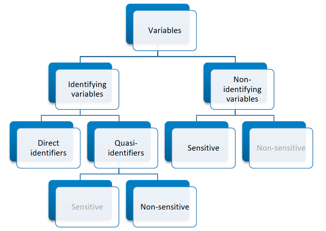
Fig. 2 Classification of variables
Disclosure scenarios
Evaluation of disclosure risk is carried out with reference to the available data sources in the environment where the dataset is to be released. In this setting, disclosure risk is the possibility of correctly re-identifying an individual in the released microdata file by matching their data to an external file based on a set of quasi-identifiers. The risk assessment is done by identifying so-called disclosure or intrusion scenarios. A disclosure scenario describes the information potentially available to the intruder (e.g., census data, electoral rolls, population registers or data collected by private firms) to identify respondents and the ways such information can be combined with the microdata set to be released and used for re-identification of records in the dataset. Typically, these external datasets include direct identifiers. In that case, the re-identification of records in the released dataset leads to identity and, possibly, attribute disclosure. The main outcome of the evaluation of disclosure scenarios is the identification of a set of quasi-identifiers (i.e., key variables) that need to be treated during the SDC process (see ELMP10).
An example of a disclosure scenario could be the spontaneous recognition of a respondent by a researcher. For instance, while going through the data, the researcher recognizes a person with an unusual combination of the variables age and marital status. Of course, this can only happen if the person is well-known or is known to the researcher. Another example of a disclosure scenario for a publicly available file would be if variables in the data could be linked to a publically available electoral register. An intruder might try matching the entire dataset with individuals in the register. However, this might be difficult and take specialized expertise, or software, and other conditions have to be fulfilled. Examples are that the point in time the datasets were collected should approximately match and the content of the variables should be (nearly) identical. If these conditions are not fulfilled, exact matching is much less likely.
Note
Not all external data is necessarily in the public domain. Also privately owned datasets or datasets which are not released should be taken into consideration for determining the suitable disclosure scenario.
Info-box - Disclosure scenarios and different release types
A dataset can have more than one disclosure scenario. Disclosure scenarios also differ depending on the data access type that the data will be released under; for example, Public Use Files (PUF) or Scientific Use Files (SUF, also known as licensed) or in a data enclave. The required level of protection, the potential avenues of disclosure as well as the availability of other external data sources differ according to the access type under which the data will be released. For example, the user of a Scientific Use File (SUF) might be contractually restricted by an agreement as to what they are allowed to do with the data, whereas a Public Use File (PUF) might be freely available on the internet under a much looser set of conditions. PUFs will in general require more protection than SUFs and SUFs will require more protection than those files only released in an data enclave. Disclosure scenarios should be developed with all of this in mind.
The evaluation of disclosure risk is based on the quasi-identifiers, which are identified in the analysis of disclosure risk scenarios. The disclosure risk directly depends on the inclusion or exclusion of variables in the set of quasi-identifiers chosen. This step in the SDC process (making the choice of quasi-identifiers) should therefore be approached with great thought and care. We will see later, as we discuss the steps in the SDC process in more detail, that the first step for any agency is to undertake an exercise in which an inventory is compiled of all datasets available in the country. Both datasets released by the national statistical office and from other sources are considered and their availability to intruders as well as the variables included in these datasets is analyzed. It is this information that will serve as a key metric when deciding which variables to choose as potential identifiers, as well as dictate the level of SDC and methods needed.
Levels of risk
With microdata from surveys and censuses, we often have to be concerned about disclosure at the individual or unit level, i.e., identifying individual respondents. Individual respondents are generally natural persons, but can also be units, such as companies, schools, health facilities, etc. Microdata files often have a hierarchical structure where individual units belong to groups, e.g., people belong to households. The most common hierarchical structure in microdata is the household structure in household survey data. Therefore, in this guide, we sometimes call disclosure risk for data with a hierarchical structure “household risk”. The concepts, however, apply equally to establishment data and other data with hierarchical structures, such as school data with pupils and teachers or company data with employees.
We will see that this hierarchical structure is important to take into consideration when measuring disclosure risk. For hierarchical data, information collected at the higher hierarchical level (e.g., household level) would be the same for all individuals in the group belonging to that higher hierarchical level (e.g., household). [3] Some typical examples of variables that would have the same values for all members of the same higher hierarchical unit are, in the case of households, those relating to housing and household income. These variables differ from survey to survey and from country to country. [4] This hierarchical structure creates a further level of disclosure risk for two reasons:
- if one individual in the household is re-identified, the household structure allows for re-identification of the other household members in the same household,
- values of variables for other household members that are common for all household members can be used for re-identification of another individual of the same household. This is discussed in more detail in the Section Household Risk.
Next, we first discuss risk measures used to evaluate disclosure risk in the absence of a hierarchical structure. This includes risk measures that seek to aggregate the individual risk for all individuals in the microdata file; the objective is to quantify a global disclosure risk measure for the file. We then discuss how risk measures change when taking the hierarchical structure of the data into account.
We will also discuss how risk measures differ for categorical and continuous key variables. For categorical variables, we will use the concept of uniqueness of combinations of values of quasi-identifiers (so-called “keys”) used to identify individuals at risk. The concept of uniqueness, however, is not useful for continuous variables, since it is likely that all or many individuals will have unique values for that variable, by definition of a continuous variable. Risk measures for categorical variables are generally a priori measures, i.e., they can be evaluated before applying anonymization methods since they are based on the principle of uniqueness. Risk measures for continuous variables are a posteriori measures; they are based on comparing the microdata before and after anonymization and are, for example, based on the proximity of observations between the original and the treated (anonymized) datasets.
Files that are limited to only categorical or only continuous key variables are easiest for risk measurement. We will see in later sections that, in cases where both types of variables are present, recoding of continuous variables into categories is one approach to use to simplify the SDC process, but we will also see that from a utility perspective this may not be desirable. An example might be the use of income quintiles instead of the actual income variables. We will see that measuring the risk of disclosure based on the categorical and continuous variables separately is generally not a valid approach.
The risk measures discussed in the next section are based on several assumptions. In general, these measures rely on quite restrictive assumptions and will often lead to conservative risk estimates. These conservative risk measures may overstate the risk as they assume a worst-case scenario. Two assumptions should, however, be fulfilled for the risk measures to be valid and meaningful; the microdata should be a sample of a larger population (no census) and the sampling weights should be available. The Section Special case: census data briefly discusses how to deal with census data.
Individual risk
Categorical key variables and frequency counts
The main focus of risk measurement for categorical quasi-identifiers is on identity disclosure. Measuring disclosure risk is based on the evaluation of the probability of correct re-identification of individuals in the released data. We use measures based on the actual microdata to be released. In general, the rarer a combination of values of the quasi-identifiers (i.e., key) of an observation in the sample, the higher the risk of identity disclosure. An intruder that tries to match an individual who has a relatively rare key within the sample data with an external dataset in which the same key exists will have a higher probability of finding a correct match than when a larger number of individuals share the same key. This can be illustrated with the following example that is illustrated in Table 1.
Table 1 shows values for 10 respondents for the quasi-identifiers “residence”, “gender”, “education level” and “labor status”. In the data, we find seven unique combinations of values of quasi-identifiers (i.e., patterns or keys) of the four quasi-identifiers. Examples of keys are {‘urban’, ‘female’, ‘secondary incomplete’, ‘employed’} and {‘urban’, ‘female’, ‘primary incomplete’, ‘non-LF’}. Let \(f_{k}\) be the sample frequency of the \(k\)th key, i.e., the number of individuals in the sample with values of the quasi-identifiers that coincide with the \(k\)th key. This would be 2 for the key {urban, female, secondary incomplete, employed}, since this key is shared by individuals 1 and 2 and 1 for the key {‘urban’, ‘female’, ‘primary incomplete’, ‘non-LF’}, which is unique to individual 3. By definition, \(f_{k}\) is the same for each record sharing a particular key.
The fewer the individuals with whom an individual shares his or her combination of quasi-identifiers, the more likely the individual is to be correctly matched in another dataset that contains these quasi-identifiers. Even when direct identifiers are removed from the dataset, that individual has a higher disclosure risk than others, assuming that their sample weights are the same. Table 1 reports the sample frequencies \(f_{k}\) of the keys for all individuals. Individuals with the same keys have the same sample frequency. If \(f_{k} = 1\), this individual has a unique combination of values of quasi-identifiers and is called “sample unique”. The dataset in Table 1 contains four sample uniques. Risk measures are based on this sample frequency.
| No | Residence | Gender | Education level | Labor status | Weight | \(f_{k}\) | \(F_{k}\) | risk |
|---|---|---|---|---|---|---|---|---|
| 1 | Urban | Female | Secondary incomplete | Employed | 180 | 2 | 360 | 0.0054 |
| 2 | Urban | Female | Secondary incomplete | Employed | 180 | 2 | 360 | 0.0054 |
| 3 | Urban | Female | Primary incomplete | Non-LF | 215 | 1 | 215 | 0.0251 |
| 4 | Urban | Male | Secondary complete | Employed | 76 | 2 | 152 | 0.0126 |
| 5 | Rural | Female | Secondary complete | Unemployed | 186 | 1 | 186 | 0.0282 |
| 6 | Urban | Male | Secondary complete | Employed | 76 | 2 | 152 | 0.0126 |
| 7 | Urban | Female | Primary complete | Non-LF | 180 | 1 | 180 | 0.0290 |
| 8 | Urban | Male | Post-secondary | Unemployed | 215 | 1 | 215 | 0.0251 |
| 9 | Urban | Female | Secondary incomplete | Non-LF | 186 | 2 | 262 | 0.0074 |
| 10 | Urban | Female | Secondary incomplete | Non-LF | 76 | 2 | 262 | 0.0074 |
For sample data, it is more interesting to look at \(F_{k}\), the population frequency of a combination of quasi-identifiers (key) \(k\), which is the number of individuals in the population with the key that corresponds to key \(k\). The population frequency is unknown if the microdata is a sample and not a census. Under certain assumptions, the expected value of the population frequencies can be computed using the sample design weight \(w_{i}\) (in a simple sample, this is the inverse of the inclusion probability) for each individual \(i\)
\(F_{k}\) is the sum of the sample weights of all records with the same key \(k\). Hence, like \(f_{k}\), \(F_{k}\) is the same for each record with key \(k\). The risk of correct re-identification is the probability that the key is matched to the correct individual in the population. Since every individual in the sample with key \(k\) corresponds to \(F_{k}\) individuals in the population, the probability of correct re-identification is \(1/F_{k}\). This is the probability of re-identification in the worst-case scenario and can be interpreted as disclosure risk. Individuals with the same key have the same frequencies, i.e., the frequency of the key.
If \(F_{k} = 1\), the key \(k\) is both a sample and a population unique and the disclosure risk would be 1. Population uniques are an important factor to consider when evaluating risk, and deserve special attention. Table 1 also shows \(F_{k}\) for the example dataset. This is further discussed in the case studies the Section Case Studies.
In practice, this approach leads to conservative risk estimates, as it does not adequately take the sampling methods into account. In this case, the estimates of re-identification risk may be estimated too high. If this overestimated risk is used, the data may be overprotected (i.e., information loss will be higher than was necessary) when applying SDC measures. Instead, a Bayesian approach to risk measurement is recommended, where the posterior distribution of \(F_{k}\) is used (see e.g., HDFG12) to estimate an individual risk measure \(r_{k}\) for each key \(k\).
ADD: more info on the exact computation of r_k
The risk measure \(r_{k}\) is, as \(f_{k}\) and \(F_{k}\), the same for all individuals sharing the same pattern of values of key variables and is referred to as individual risk. The values \(r_{k}\) can also be interpreted as the probability of disclosure for the individuals or as the probability for a successful match with individuals chosen at random from an external data file with the same values of the key variables. This risk measure is based on certain assumptions [5], which are strict and may lead to a relatively conservative risk measure. The risk measures are also presented in Table 1.
The main factors influencing the individual risk are the sample frequencies \(f_{k}\) and the sampling design weights \(w_{i}\). If an individual is at relatively high risk of disclosure, in our example this would be individuals 3, 5, 7 and 8 in Table 1, the probability that a potential intruder correctly matches these individuals with an external data file is high relative to the other individuals in the released data. In our example, the reason for the high risk is the fact that these individuals are sample uniques \((f_{k} = 1)\). This risk is the worst-case scenario risk and does not imply that the person will be re-identified with certainty with this probability. For instance, if an individual included in the microdata is not included in the external data file, the probability for a correct match is zero. Nevertheless, the risk measure computed based on the frequencies will be positive.
\(k\)-anonymity
The risk measure \(k\)-anonymity is based on the principle that, in a safe dataset, the number of individuals sharing the same combination of values (keys) of categorical quasi-identifiers should be higher than a specified threshold \(k\). \(k\)-anonymity is a risk measure based on the microdata to be released, since it only takes the sample into account. An individual violates \(k\)-anonymity if the sample frequency count \(f_{k}\) for the key \(k\) is smaller than the specified threshold \(k\). For example, if an individual has the same combination of quasi-identifiers as two other individuals in the sample, these individuals satisfy 3-anonymity but violate 4-anonymity. In the dataset in Table 1, six individuals satisfy 2-anonymity and four violate 2-anonymity. The individuals that violate 2-anonymity are sample uniques. The risk measure is the number of observations that violates k-anonymity for a certain value of k, which is
where \(I\) is the indicator function and \(i\) refers to the \(i\)th record. This is simply a count of the number of individuals with a sample frequency of their key lower than \(k\). The count is higher for larger \(k\), since if a record violates \(k\)-anonymity, it also violates \((k + 1)\)-anonymity. The risk measure \(k\)-anonymity does not consider the sample weights, but it is important to consider the sample weights when determining the required level of \(k\)-anonymity. If the sample weights are large, one individual in the dataset represents more individuals in the target population, the probability of a correct match is smaller, and hence the required threshold can be lower. Large sample weights go together with smaller datasets. In a smaller dataset, the probability to find another record with the same key is smaller than in a larger dataset. This probability is related to the number of records in the population with a particular key through the sample weights.
Assuming that the example dataset in Table 1 represents the full sample, we find that four observations violate 2-anonymity (\(f_{k} < 2\)) and all 10 observations violate 3-anonymity (\(f_{k} < 3\)). The relative number of 2-anonymity and 3-anonymity violators are resp. 40% and 100%. For other levels of \(k\)-anonymity, it is possible to compute the number of violating individuals by using the sample frequency counts. \(k\) can be replaced with any required threshold. The choice of the required threshold that all individuals in the microdata file should satisfy depends on many factors and is discussed further in the Section Local suppression on local suppression. In many institutions, typically required thresholds for \(k\)-anonymity are 3 and 5.
It is important to note that missing values are treated as if they were any other value. Two individuals with keys {‘Male’, missing, ‘Employed’} and {‘Male’, ‘Secondary complete’, ‘Employed’} share the same key, and similarly, {‘Male’, missing, ‘Employed’} and {‘Male’, ‘Secondary incomplete’, ‘Employed’} also share the same key. Therefore, the missing value in the first key is first interpreted as ‘Secondary complete’, and then as ‘Secondary incomplete’. This is illustrated in Table 2.
Note
The sample frequency of the third record is 3, since it is regarded to share its key both with the first and second record.
This principle is used when applying local suppression to achieve a certain level of \(k\)-anonymity (see the Section Local suppression) and is based on the fact that the value NA could replace any value.
ADD: parameter alpha and treating missing values
| No | Gender | Education level | Labor status | \(f_{k}\) |
|---|---|---|---|---|
| 1 | Male | Secondary complete | Employed | 2 |
| 2 | Male | Secondary incomplete | Employed | 2 |
| 3 | Male | NA | Employed | 3 |
If a dataset satisfies \(k\)-anonymity, an intruder will always find at least \(k\) individuals with the same combination of quasi-identifiers. \(k\)-anonymity is often a necessary requirement for anonymization for a dataset before release, but is not necessarily a sufficient requirement. The \(k\)-anonymity measure is only based on frequency counts and does not take (differences in) sample weights into account. Often \(k\)-anonymity is achieved by first applying recoding and subsequently applying local suppression, and in some cases by microaggregation, before using other risk measures and disclosure methods to further reduce disclosure risk. These methods are discussed in the Section Anonymization methods.
\(l\)-diversity
\(k\)-anonymity has been criticized for not being restrictive enough. Sensitive information might be disclosed even if the data satisfies \(k\)-anonymity. This might occur in cases where the data contains sensitive (non-identifying) categorical variables that have the same value for all individuals that share the same key. Examples of such sensitive variables are those containing information on an individual’s health status. Table 3 illustrates this problem by using the same data as previously used, but adding a sensitive variable, ”health”. The first two individuals satisfy 2-anonymity for the key variables “residence”, “gender”, “education level” and “labor status”. This means that an intruder will find at least two individuals when matching to the released microdata set based on those four quasi-identifiers. Nevertheless, if the intruder knows that someone belongs to the sample and has the key {‘Urban’, ‘Female’, ‘Secondary incomplete’ and ‘Employed’}, with certainty the health status is disclosed (‘yes’), because both observations with this key have the same value. This information is thus disclosed without the necessity to match exactly to the individual. This is not the case for the individuals with the key {‘Urban’, ‘Male’, ‘Secondary complete’, ‘Employed’}. Individuals 4 and 6 have different values (‘yes’ and ‘no’) for “health”, and thus the intruder would not gain information about the health status from this dataset by matching an individual to one of these individuals.
| No | Residence | Gender | Education level | Labor status | Health | \(f_{k}\) | \(F_{k}\) | \(l\)-diversity |
|---|---|---|---|---|---|---|---|---|
| 1 | Urban | Female | Secondary incomplete | Employed | yes | 2 | 360 | 1 |
| 2 | Urban | Female | Secondary incomplete | Employed | yes | 2 | 360 | 1 |
| 3 | Urban | Female | Primary incomplete | Non-LF | yes | 1 | 215 | 1 |
| 4 | Urban | Male | Secondary complete | Employed | yes | 2 | 152 | 2 |
| 5 | Rural | Female | Secondary complete | Unemployed | yes | 1 | 186 | 1 |
| 6 | Urban | Male | Secondary complete | Employed | no | 2 | 152 | 2 |
| 7 | Urban | Female | Primary complete | Non-LF | no | 1 | 180 | 1 |
| 8 | Urban | Male | Post-secondary | Unemployed | yes | 1 | 215 | 1 |
| 9 | Urban | Female | Secondary incomplete | Non-LF | no | 2 | 262 | 2 |
| 10 | Urban | Female | Secondary incomplete | Non-LF | yes | 2 | 262 | 2 |
The concept of (distinct) \(l\)-diversity addresses this shortcoming of \(k\)-anonymity (see MKGV07). A dataset satisfies \(l\)-diversity if for every key \(k\) there are at least \(l\) different values for each of the sensitive variables. In the example, the first two individuals satisfy only 1-diversity, individuals 4 and 6 satisfy 2-diversity. The required level of \(l\)-diversity depends on the number of possible values the sensitive variable can take. If the sensitive variable is a binary variable, the highest level if \(l\)-diversity that can be achieved is 2. A sample unique will always only satisfy 1-diversity.
ADD: recursive l-diversity and parameter l_recurs_c in ldiversity()
\(l\)-diversity is useful if the data contains categorical sensitive variables that are not quasi-identifiers themselves. It is not possible to select quasi-identifiers to calculate the \(l\)-diversity. \(l\)-diversity has to be calculated for each sensitive variable separately.
Special Uniques Detection Algorithm (SUDA)
The previously discussed risk measures depend on identifying key variables for which there may be information available from other sources or other datasets, and which, when combined with the current data, may lead to re-identification. In practice, however, it might not always be possible to conduct an inventory of all available datasets and their variables and thus assess all known external linkages and risks.
To overcome this, an alternative heuristic measure based on special uniques has been developed to determine the riskiness of a record, which leads to a SUDA metric or score (see ElMF02). These measures are based on the search for special uniques. To find these special uniques, algorithms, called SUDA (Special Uniqueness Detection Algorithm), have been developed. SUDA algorithms are based on the concept of special uniqueness, which is introduced in the next subsection. Since this is a heuristic approach, its performance is only tested in actual datasets, which is done in ElMF02 for UK census data. These tests have shown that the performance of the algorithm leads to good risk estimates for these test datasets.
Sample unique vs. special unique
The previous measures of risk focused on the uniqueness of the key of a record in the dataset. Table 4 reproduces the data from Table 1. The sample dataset has 10 records and four pre-determined quasi-identifiers {“Residence”, “Gender”, “Education level” and “Labor status”}. Given the four quasi-identifiers, we have seven distinct patterns in those key variables, or keys (e.g., {‘Urban’, ‘Female’, ‘Secondary incomplete’, ‘Employed’}). The sample frequency counts of the first and second records equal 2, because the two records share the same pattern (i.e., {‘Urban’, ‘Female’, ‘Secondary incomplete’, ‘Employed’}). Record 3 is a sample unique because it is the only individual in the sample who is a female living in an urban area who is employed without completing primary school. Similarly, records 5, 7 and 8 are sample uniques, because they possess distinct patterns with respect to the four key variables.
| No | Residence | Gender | Education level | Labor status | Weight | \(f_{k}\) | \(F_{k}\) | risk |
|---|---|---|---|---|---|---|---|---|
| 1 | Urban | Female | Secondary incomplete | Employed | 180 | 2 | 360 | 0.0054 |
| 2 | Urban | Female | Secondary incomplete | Employed | 180 | 2 | 360 | 0.0054 |
| 3 | Urban | Female | Primary incomplete | Non-LF | 215 | 1 | 215 | 0.0251 |
| 4 | Urban | Male | Secondary complete | Employed | 76 | 2 | 152 | 0.0126 |
| 5 | Rural | Female | Secondary complete | Unemployed | 186 | 1 | 186 | 0.0282 |
| 6 | Urban | Male | Secondary complete | Employed | 76 | 2 | 152 | 0.0126 |
| 7 | Urban | Female | Primary complete | Non-LF | 180 | 1 | 180 | 0.0290 |
| 8 | Urban | Male | Post-secondary | Unemployed | 215 | 1 | 215 | 0.0251 |
| 9 | Urban | Female | Secondary incomplete | Non-LF | 186 | 2 | 262 | 0.0074 |
| 10 | Urban | Female | Secondary incomplete | Non-LF | 76 | 2 | 262 | 0.0074 |
In addition to the records 3, 5, 7 and 8 in Table 4 being sample uniques with respect to the key variable set {“Residence”, “Gender”, “Education level”, “Labor status”}, we can find unique patterns in these records without even having to consider the complete set of key variables. For instance, a unique pattern can be found in record 5 when we look only at the variables “Education level” and “Labor status” ({‘Secondary complete’, ‘Unemployed’}). While the values {‘Secondary complete’} and {‘Unemployed’} are not unique in the sample, the combination of them, {‘Secondary complete’, ‘Unemployed’} makes record 5 unique. This variable subset is referred to as the Minimal Sample Unique (MSU) as any smaller subset of this set of variables is not unique (in this case {‘Secondary complete’} and {‘Unemployed’}). It is an MSU of size 2. This holds as well for three other combinations in record 5, i.e., {‘Female’, ‘Unemployed’} and {‘Female’, ‘Secondary Complete’}, which are also MSUs of size 2 and {‘Rural’} of size 1. In total, record 5 has four MSUs [7]. To determine if a set is an MSU of size \(k\), we check whether it fulfills the minimal requirement. It suffices to check whether all subsets of size \(k-1\) of the MSU are unique. If any of these subsets are also unique in the sample, the set found may be a sample unique, but violates the minimal requirement and is hence not an MSU. The unique subset of size \(k-1\) could be a MSU. In our example, to determine if the MSU {‘Secondary complete’, ‘Unemployed’} is a MSU, we checked as to whether its subsets {‘Secondary complete’} and {‘Unemployed’} were not unique in the sample. By definition, only sample uniques can be special uniques.
The SUDA algorithm identifies all the MSUs in the sample, which in turn are used to assign a SUDA score to each record. This score indicates how “risky” a record is. The potential risk of the records is determined based on two observations:
- The smaller the size of the MSU within a record (i.e., the fewer variables are needed to reach uniqueness), the greater the risk of the record
- The larger the number of MSUs possessed by a record, the greater the risk of the record
A record is defined as a special unique if it is a sample unique both on the complete set of quasi-identifiers (e.g., in the data in Table 4, the variables “Residence”, ”Gender”, “Education level” and “Labor status”) and simultaneously has at least one MSU (ElSD98). Special uniques can be classified according to the number and size of subsets that are MSUs. Research has shown that special uniques are more likely to be population uniques than random uniques (ElMF02) and are thus relevant for risk assessment.
Calculating SUDA scores
The SUDA algorithm is used to search for MSUs in the data among the sample uniques to determine which sample uniques are also special uniques i.e., have subsets that are also unique (see Elliot et al., 2005). First the SUDA algorithm is used to identify the MSUs for each sample unique. To simplify the search and because smaller subsets are more important for disclosure risk, the search is limited to a maximum subset size. Subsequently, a score is assigned to each individual, which ranks the individuals according to their level of risk.
For each MSU of size \(k\) contained in a given record, a score is computed by \(\prod_{i = k}^{M}{(ATT - i)}\), where \(M\) is the user-specified maximum size of MSUs [8], and \(ATT\) is the total number of attributes or variables in the dataset. By definition, the smaller the size \(k\) of the MSU, the larger the score for the MSU, which reflects greater risk (see EMMG05). The final SUDA score for each record is computed by adding the scores for each MSU in the record. In this way, records with more MSUs are assigned a higher SUDA score, which also reflects the higher risk. The SUDA score ranks the individuals according to their level of risk. The higher the SUDA score, the riskier the sample unique.
Calculating SUDA scores – a simplified example
To illustrate how SUDA scores are calculated, we compute the SUDA scores for the sample uniques in the data in Table 5, which replicates the data from Table 5. Record 5 contains four MSUs: {Rural} of size 1, and {‘Secondary Complete’, ‘Unemployed’}, {‘Female’, ‘Unemployed’} and {Female, Secondary Complete} of size 2. Suppose the maximum size of MSUs we search for in the data, \(M\), is set at 3. Knowing that, \(ATT\), the number of selected key variables in the dataset, is 4; the score assigned to {Rural} is computed by \(\prod_{i = 1}^{3}{(4 - i)} = 3*2*1 = 6\); and the score assigned to {Secondary complete, Unemployed}, {Female, Unemployed} and {Female, Secondary Complete} is \(\prod_{i = 2}^{3}\left( 4 - i \right) = 2*1 = 2\). The SUDA score for the fifth record in Table 5 is then \(6 + 2 + 2 + 2 = 12\), which is the sum of these four scores per MSU. The SUDA scores for the other sample uniques are computed accordingly [9]. The values that are in the MSUs in the sample uniques are shaded in Table 5. Records that are not sample uniques (\(f_{k} > 1\)) cannot be special uniques and are assigned the score 0.
| No | Residence | Gender | Education level | Labor status | Weight | \(f_{k}\) | SUDA score | DIS-SUDA |
|---|---|---|---|---|---|---|---|---|
| 1 | Urban | Female | Secondary incomplete | Employed | 180 | 2 | 0 | 0.0000 |
| 2 | Urban | Female | Secondary incomplete | Employed | 180 | 2 | 0 | 0.0000 |
| 3 | Urban | Female | Primary incomplete | Non-LF | 215 | 1 | 6 | 0.0051 |
| 4 | Urban | Male | Secondary complete | Employed | 76 | 2 | 0 | 0.0000 |
| 5 | Rural | Female | Secondary complete | Unemployed | 186 | 1 | 12 | 0.0107 |
| 6 | Urban | Male | Secondary complete | Employed | 76 | 2 | 0 | 0.0000 |
| 7 | Urban | Female | Primary complete | Non-LF | 180 | 1 | 6 | 0.0051 |
| 8 | Urban | Male | Post-secondary | Unemployed | 215 | 1 | 10 | 0.0088 |
| 9 | Urban | Female | Secondary incomplete | Non-LF | 186 | 2 | 0 | 0.0000 |
| 10 | Urban | Female | Secondary incomplete | Non-LF | 76 | 2 | 0 | 0.0000 |
ADD: compare with values in code block 4.7
To estimate record-level disclosure risks, SUDA scores can be used in combination with the Data Intrusion Simulation (DIS) metric (ElMa03), a method for assessing disclosure risks for the entire dataset (i.e., file-level disclosure risks). Roughly speaking, the DIS-SUDA method distributes the file-level risk measure generated by the DIS metric between records according to the SUDA scores of each record. This way, SUDA scores are calibrated against a consistent measure to produce the DIS-SUDA scores, which provide the record-level disclosure risk. These scores are used to compute the conditional probability that a unique match found by an intruder between the sample unique in the released microdata and an external data source is also a correct match, and hence a successful disclosure. The DIS-SUDA measure can be computed in sdcMicro. Since the DIS score is a probability, its values are in the interval \(\lbrack 0,\ 1\rbrack\). A full description of the DIS-SUDA method is provided by ElMa03.
Note that unlike the risk methods discussed earlier, the DIS-SUDA score does not fully account for the sampling weights. Risk measures based on the previous methods (i.e., negative binomial models) will in general have lower risks for those records with greater sampling weight, given the same sample frequency count, than those measured using DIS-SUDA. Therefore, instead of replacing the risk measures introduced in the previous section, the SUDA scores and DIS-SUDA approach should be used as a complementary method. As mentioned earlier, DIS-SUDA is particularly useful in situations where taking an inventory of all already available datasets and their variables is difficult.
ADD: why use SUDA: (Typically, after applying SDC methods, one would recalculate the SUDA scores and compare them to the original values. One way to quickly see the differences would be to rerun these visualizations and compare them to the base for risk changes.)
ADD: reference to fig2

Fig. 3 Visualizations of DIS-SUDA scores
Risk measures for continuous variables
The principle of rareness or uniqueness of combinations of quasi-identifiers (keys) is not useful for continuous variables, because it is likely that all or many individuals will have unique keys. Therefore, other approaches are exploited for measuring the disclosure risk of continuous variables. These methods are based on uniqueness of the values in the neighborhood of the original values. The uniqueness is defined in different ways: in absolute terms (interval measure) or relative terms (record linkage). Most measures are a posteriori measures: they are evaluated after anonymization of the raw data, compare the treated data with the raw data and evaluate for each individual the distance between the values in the raw and the treated data. This means that these methods are not useful for identifying individuals at risk within the raw data, but rather show the distance/difference between the dataset before and after anonymization and can therefore be interpreted as evaluation of the anonymization method. For that reason, they resemble the information loss measures discussed in the Section Measuring utility and information loss. Finally, risk measures for continuous quasi-identifiers are also based on outlier detection. Outliers play an important role in the re-identification of these records.
Record linkage
Record linkage is an a posteriori method that evaluates the number of correct linkages when linking the perturbed values with the original values. The linking algorithm is based on the distance between the original and the perturbed values (i.e., distance-based record linkage). The perturbed values are matched with the closest individual. It is important to note that this method does not give information on the initial risk, but is rather a measure to evaluate the perturbation algorithm (i.e., it is designed to indicate the level of uncertainty introduced into the variable by counting the number of records that could be correctly matched).
Record linkage algorithms differ with respect to which distance measure is used. When a variable has very different scaling than other continuous variables in the dataset, rescaling the variables before using record linkage is recommended. Very different scales may lead to undesired results when measuring the multivariate distance between records based on several continuous variables. Since these methods are based on both the raw data and treated data, examples of their applications require the introduction of SDC methods and are therefore postponed to the case studies in the Section Case Studies.
Besides distance-based record linkage, another method for linking is probabilistic record linkage (see DoTo03). The literature shows, however, that results from distance-based record linkage are better than the results from probabilistic record linkage. Individuals in the treated data that are linked to the correct individuals in the raw data are considered at risk of disclosure.
Interval measure
Successful application of an SDC method should result in perturbed values that are considered not too close to their initial values; if the value is relatively close, re-identification may be relatively easy. In the application of interval measures, intervals are created around each perturbed value and then a determination is made as to whether the original value of that perturbed observation is contained in this interval. Values that are within the interval around the initial value after perturbation are considered too close to the initial value and hence unsafe and need more perturbation. Values that are outside of the intervals are considered safe. The size of the intervals is based on the standard deviation of the observations and a scaling parameter \(k\).
ADD: size of interval
The size of the intervals is \(k\) times the standard deviation. The larger \(k\), the larger the intervals are, and hence the larger the number of observations within the interval constructed around their original values and the higher the risk measure.
For most values, this is a satisfactory approach. It is not a sufficient measure for outliers, however. After perturbation, outliers will stay outliers and are easily re-identifiable, even if they are sufficiently far from their initial values. Therefore, outliers should be treated with caution.
Outlier detection
Outliers are important for measuring re-identification risk in continuous microdata. Continuous data are often skewed, especially right-skewed. This means that there are a few outliers with very high values relative to the other observations of the same variable. Examples are income in household data, where only few individuals/households may have very high incomes, or turnover data for firms that are much larger than other firms in the sample are. In cases like these, even if these values are perturbed, it may still be easy to identify these outliers, since they will stay the largest values even after perturbation. (The perturbation will have created uncertainty as to the exact value, but because the value started out so much further away from other observations, it may still be easy to link to the high-income individual or very large firm.) Examples would be the only doctor in a geographical area with a high income or one single large firm in one industry type. Therefore, identifying outliers in continuous data is an important step when identifying individuals at high risk. In practice, identifying the values of a continuous variable that are larger than a predetermined \(p\%\)-percentile might help identify outliers, and thus units at greater risk of identification. The value of \(p\) depends on the skewness of the data.
A second approach for outlier detection is a posteriori measure comparing the treated and raw data. An interval is constructed around the perturbed values as described in the previous section. If the original values fall into the interval around the perturbed values, the perturbed values are considered unsafe since they are too close to the original values. There are different ways to construct such intervals, such as rank-based intervals and standard deviation-based intervals. TeMe08 propose a robust alternative for these intervals. They construct the intervals based on the squared Robust Mahalanobis Distance (RMD) of the individual values. The intervals are scaled by the RMD such that outliers obtain larger intervals and hence need to have a larger perturbation in order to be considered safe than values that are not outliers. This method is illustrated in the Section Case Studies.
Global risk
To construct one aggregate risk measure at the global level for the complete dataset, we can aggregate the measures for risk at the individual level in several ways. Global risk measures should be used with caution: behind an acceptable global risk can hide some very high-risk records that are compensated by many low risk records.
Mean of individual risk measures
A straightforward way of aggregating the individual risk measures is taking the mean of all individuals in the sample, which is equal to summing over all keys in the sample if multiplied by the sample frequencies of these keys and dividing by the sample size \(n\):
\(r_{k}\) is the individual risk of key \(k\) that the \(i\)th individual shares (see the Section Categorical key variables and frequency counts).
The global risk in the example data in Table 1 is 0.01582, which is the expected proportion of all individuals in the sample that could be re-identified by an intruder. Another way of expressing the global risk is the number of expected re-identifications, \(n*R_{1}\), which is in the example 10 * 0.01582.
Note
This global risk measure should be used with caution. The average risk can be relatively low, but a few individuals could have a very high probability of re-identification.
An easy way to check for this is to look at the distribution of the individual risk values or the number of individuals with risk values above a certain threshold, as shown in the next section.
Count of individuals with risks larger than a certain threshold
All individuals belonging to the same key have the same individual risk, \(r_{k}\). Another way of expressing the total risk in the sample is the total number of observations that exceed a certain threshold of individual risk. Setting the threshold can be absolute (e.g., all those individuals who have a disclosure risk higher than 0.05 or 5%) or relative (e.g., all those individuals with risks higher than the upper quartile of individual risk). In the example, no individual has a higher disclosure risk than 0.05.
These calculations can then be used to treat data for individuals whose risk values are above a predetermined threshold. For example, one could suppress values of certain key variables for those individuals with risk above a specified threshold. This is explained further in the Section Local suppression .
Household risk
In many social surveys, the data have a hierarchical structure where an individual belongs to a higher-level entity (see the Section Levels of risk). Typical examples are households in social surveys or pupils in schools. Re-identification of one household member can lead to re-identification of the other household members, too. It is therefore easy to see that if we take the household structure into account, the re-identification risk is the risk that at least one of the household members is re-identified.
where \(A_{j}\) is the event that the \(j\)th member of the household is re-identified and \(P\left( A_{j} \right) = r_{k}\) is the individual disclosure risk of the \(j\)th member. For example, if a household member has three members with individual disclosure risks based on their respective keys 0.02, 0.03 and 0.03, respectively, the household risk is
The hierarchical or household risk cannot be lower than the individual risk, and the household risk is always the same for all household members. The household risk should be used in cases where the data contain a hierarchical structure, i.e., where a household structure is present in the data.
Note
The size of a household is an important identifier itself, especially for large households. Suppression of the actual size variable (e.g., number of household members), however, does not suffice to remove this information from the dataset, as a simple count of the household members for a particular household will allow reconstructing this variable as long as a household ID is in the data, which allows assigning individuals to households. We flag this for the reader’s attention as it is important. Further discussion on approaches to the SDC process that take into account the household structure where it exists can be found in the Section Anonymization of the quasi-identifier household size
Recommended Reading Material on Risk Measurement
Elliot, Mark J, Anna Manning, Ken Mayes, John Gurd, and Michael Bane. 2005. “SUDA: A Program for Detecting Special Uniques.” Joint UNECE/Eurostat Work Session on Statistical Data Confidentiality. Geneva.
Hundepool, Anco, Josep Domingo-Ferrer, Luisa Franconi, Sarah Giessing, Eric Schulte Nordholt, Keith Spicer, and Peter Paul de Wolf. 2012. Statistical Disclosure Control. Chichester: John Wiley & Sons Ltd. doi:10.1002/9781118348239.
Lambert, Diane. 1993.”Measures of Disclosure Risk and Harm.” Journal of Official Statistics 9(2) : 313-331.
Machanavajjhala, Ashwin, Daniel Kifer, Johannes Gehrke, and Muthuramakrishnan Venkitasubramaniam. 2007. “L-diversity: Privacy Beyond K-anonymity.” ACM Trans. Knowl. Discov. Data 1 (Article 3) (1556-4681). doi:10.1145/1217299.1217302. https://ptolemy.berkeley.edu/projects/truststc/pubs/465/L%20Diversity%20Privacy.pdf. Accessed July 6, 2018.
Templ, Matthias, Bernhard Meindl, Alexander Kowarik, and Shuang Chen. 2014. “Introduction to Statistical Disclosure Control (SDC).” http://www.ihsn.org/home/sites/default/files/resources/ihsn-working-paper-007-Oct27.pdf. August 1. Accessed July 6, 2018.
| [1] | Recoding a continuous variable is sometimes useful in cases where the data contains only a few continuous variables. We will see in the Section Individual risk that many methods used for risk calculation depend on whether the variables are categorical. We will also see that it is easier for the measurement of risk if the data contains only categorical or only continuous variables. |
| [2] | This is discussed in greater detail in the following sections. In cases where the number of possible values is large, recoding the variable, or parts of the set it takes values on, to obtain fewer distinct values is recommended. |
| [3] | Besides variables collected at the higher hierarchical level, also variables collected at the lower level but with no (or little) variation within the groups formed by the hierarchical structure should be treated as higher level variables. An example could be mother tongue, where most households are monolingual, but the variable is collected at the individual level. |
| [4] | Religion, for example, can be shared by all household members in some countries, whereas in other countries this variable is measured at the individual level and mixed-religion households exist. |
| [5] | The assumptions for this risk measure are strict and the risk is estimated in many cases higher than the actual risk. Among other assumptions, it is assumed that all individuals in the sample are also included in the external file used by the intruder to match against. If this is not the case, the risk is much lower; if the individual in the released file is not contained in the external file, the probability of a correct match is zero. Other assumptions are that the files contain no errors and that both sets of data were collected simultaneously, i.e. they contain the same information. These assumptions will often not hold generally, but are necessary for computation of a measure. An example of a violation of the last assumptions is could occur if datasets are collected at different points in time and records have changed. This could happen when people move or change jobs and makes correct matching impossible. The assumptions assume a worst-case scenario. |
| [6] | Besides distinct \(l\)-diversity, there are other \(l\)-diversity methods: entropy and recursive. Distinct \(l\)-diversity is most commonly used. |
| [7] | There are more combinations of quasi-identifiers that make record 5 unique (e.g., {‘Rural’, ‘Female’} and {‘Female’, ‘Secondary Complete’, ‘Unemployed’}. These combinations, however, are not considered MSUs because they do not fulfill the minimal subset requirement. They contain subsets that are MSUs. |
| [8] | OECD, http://stats.oecd.org/glossary |
| [9] | The third record has one MSU, {‘Primary incomplete’}; the seventh record has one MSU, {‘Primary complete’}; and the eighth record has three MSUs, {‘Urban, Unemployed’}, {‘Male, Unemployed’} and {‘Post-secondary’}. |
References
| [DoTo03] | Domingo-Ferrer, J., & Torra, V. (2003). Disclosure Risk Assesment in Statistical Microdata Protection via Advanced Record Linkage. Statistics and Computing 13 (4), 343-354 |
| [ElMa03] | Elliot , M. J., & Manning, A. M. (2003). Using DIS to Modify the Classification of Special Uniques. Invited Paper. Joint ECE/Eurostat Work Session on Statistical Data Confidentiality. Luxemboug 2-9 April 2003. |
| [ElMF02] | Elliot, M. J., Manning, A. M., & Ford, R. W. (2002). A Computational Algorithm for Handling the Special Uniques Problem. International Journal of Uncertainty, Fuzziness and Knowledge Based System , 10 (5), 493-509. |
| [ELMP10] | Elliot, M. J., Lomax, S., Mackey, E. & Purdam, K. (2010) Data Environment Analysismand the Key Variable Mapping System. In Privacy in Databases, PSD 2010 (ed. Domingo-Ferrer, J. & Magkos, E.), vol. 6344 of Lecture Notes in Computer Science, pp. 138-145. Berlin/Heidelberg: Springer |
| [ElSD98] | Elliot, M.J., Skinner, C.J. & Dale, A. (1998) Special Uniques, Random Uniques, and Sticky Populations: Some Counterintuitive Effects of Geographical Detail on Disclosure Risk Reasearch in Official Statistics 1(2), pp. 53-67 |
| [EMMG05] | Elliot, M. J., Manning, A., Mayes, K., Gurd, J., & Bane, M. (2005). SUDA: A Program for Detecting Special Uniques. Joint UNECE/Eurostat Work Session on Statistical Data Confidentiality. Geneva. |
| [HDFG12] | Hundepool, A., Domingo-Ferrer, J., Franconi, L., Giessing, S., Nordholt, E. S., Spicer, K., et al. (2012). Statistical Disclosure Control. Chichester, UK: John Wiley & Sons Ltd. |
| [Lamb93] | Lambert, D. (1993). Measures of Disclosure Risk and Harm. Journal of Official Statistics , 9 (2), 313-331. |
| [MaHK08] | Manning, A. M., Haglin, D. J., & Keane, J. A. (2008). A Recursive Search Algorithm for Statistical Disclosure Assessment. Data Mining and Knowledge Discovery , 16 (2), 165-196. |
| [MKGV07] | Machanavajjhala, A., Kifer, D., Gehrke, J., & Venkitasubramaniam, M. (2007). L-diversity: Privacy Beyond K-anonymity. ACM Trans. Knowl. Discov. Data , 1 (Article 3) (1556-4681). |
| [TeMe08] | Templ, M. & Meindl, B. (2008) Robust Statistics Meets SDC: New Disclosure Risk Measures for Continuous Microdata Masking. In Privacy in Statistical Databases, PSD 2008 (eds. Domingo-Ferrer J. and Saygin Y.), vol. 5262 of Lecture Notes in Computer Science, pp. 177-189. Berlin/Heidelberg: Springer. |
| [TeMK14] | Templ, M., Meindl, B., & Kowarik, A. (2014, August). Tutorial for SDCMicroGUI. Retrieved from International Household Survey Network (IHSN): http://www.ihsn.org/home/software/disclosure-control-toolbox |
| [TMKC14] | Templ, M., Meindl, B., Kowarik, A., & Chen, S. (2014, August 1). Introduction to Statistical Disclosure Control (SDC). Retrieved November 13, 2014, from http://www.ihsn.org/home/software/disclosure-control-toolbox. |