Case Studies (Illustrating the SDC Process)

In order to evaluate the use of different SDC methods on different types of survey datasets, we compared the results of the different methods applied to 75 datasets from 52 countries representing six geographic regions: Latin America and the Caribbean (LAC), Sub-Saharan Africa (AFR), South Asia (SA), Europe and Central Asia (ECA), Middle East and North Africa (MENA) as well as East Asia and the Pacific (EAP). The datasets chosen were from a mix of datasets that are already publically available, as well as data made available to the World Bank. The surveys used included, amongst others, household, demographic, and health surveys. The variables from these surveys used for the experiments were selected based on their relevance for users (e.g., for indicators, MDGs), their sensitivity, and their classification with respect to the SDC process.

The following case studies draw from knowledge gained from these experiments and try to incorporate the lessons learned. The case studies use synthetic data that mimic the structure of the survey types we used in our experiments and present the anonymization of a dataset similar to many surveys designed to measure household income and consumption, labor force participation and general demographic characteristics. The first case study creates a SUF, whereas in the second case study we take this SUF and treat it further to create a PUF.

Case study 1- SUF

This case study shows an example of how the anonymization process might be approached, particularly for a dataset with many continuous variables. We also show how this can be achieved using the open source and free sdcMicro package and R. A ready-to-run R script for this case study and the dataset are also available to reproduce the results and allow the user to adapt the code (see http://ihsn.org/home/projects/sdc-practice). Extracts of this code are presented in this section to illustrate several steps of the anonymization process.

Note

The choices of methods and parameters in this case study are based on this particular dataset and the results and choices might be different for other datasets.

The aim is to show the process, not to compare methods per se.

This example uses a dataset with a similar structure to that of a typical social survey with a focus on demographics, labor force participation and income and expenditure patterns. The dataset has been compiled using observations from several datasets from different countries. They are considered synthetic data and as such are used only for illustrative purposes. The source datasets were already treated for disclosure control by their producers. This does not matter, as our concern is to illustrate the process only. The data from which we compiled our case study file was from surveys that contain many variables, but pay particular attention to labor force variables as well as household income and household expenditure variables. The variables in the demo dataset have already been pre-selected from the total set of variables available in the datasets. See Appendix A for the complete overview of all variables.

This case study follows the steps of the SDC process outlined in the Section The SDC Process.

Step 1: Need for disclosure control

The statistical units in this dataset are individuals and households. The household structure provides a hierarchical structure in the data, which should be taken into account when measuring risk and selecting anonymization methods.

The data contains variables with demographic information, income, expenditures, education variables and variables relating to the labor status of the individual. These variables include sensitive and confidential variables. The dataset is an example of a social survey and, due to the nature of the statistical units and the variables, disclosure control is needed before release of the microdata. This is the case regardless of the legal framework, which is not specified here, as this is a hypothetical dataset.

Step 2: Data preparation and exploring data characteristics

The first step is to explore the data. To analyze the data in R we first have to read the data into R. In our case, the data is saved in a STATA file (.dta file). To read STATA files, we need to load the R package foreign (see the Section Read functions in R on importing other data formats in R). We also load the sdcMicro package and several other packages used later for the computation of the utility measures. If these packages are not yet installed, you should do so before trying to load them. The R code for this case study demonstrates how to do this.

Listing 1 Loading required packages

# Load required packages
library(foreign)   # for read/write function for STATA files
library(sdcMicro)  # sdcMicro package with functions for the SDC process
library(laeken)    # for GINI
library(reldist)   # for GINI
library(bootstrap) # for bootstrapping
library(ineq)      # for Lorenz curves

After setting the working directory to the directory where the STATA file is stored, we load the data into the object called file. All output, unless otherwise specified, is saved in the working directory.

Listing 2 Loading the data

#  Set working directory
setwd("C:/WorldBank/CaseStudy/")

# Specify file name
fname <- " case_1_data.dta"

# Read-in file
file <- read.dta(fname, convert.factors = F) # factors as numeric code

We check the number of variables, number of observations and variable names, as shown in Listing 3.

Listing 3 Number of individuals and variables and variable names

dim(file) # Dimensions of file (observations, variables)
## [1] 10574 68

colnames(file) # Variable names
##  [1] "REGION"        "DIST"          "URBRUR"        "WGTHH"
##  [5] "WGTPOP"        "IDH"           "IDP"           "HHSIZE"
##  [9] "GENDER"        "REL"           "MARITAL"       "AGEYRS"
## [13] "AGEMTH"        "RELIG"         "ETHNICITY"     "LANGUAGE"
## [17] "MORBID"        "MEASLES"       "MEDATT"        "CHWEIGHTKG"
## [21] "CHHEIGHTCM"    "ATSCHOOL"      "EDUCY"         "EDYRS"
## [25] "EDYRSCURRAT"   "SCHTYP"        "LITERACY"      "EMPTYP1"
## [29] "UNEMP1"        "INDUSTRY1"     "EMPCAT1"       "WHOURSWEEK1"
## [33] "OWNHOUSE"      "ROOF"          "TOILET"        "ELECTCON"
## [37] "FUELCOOK"      "WATER"         "OWNAGLAND"     "LANDSIZEHA"
## [41] "OWNMOTORCYCLE" "CAR"           "TV"            "LIVESTOCK"
## [45] "INCRMT"        "INCWAGE"       "INCBONSOCALL"  "INCFARMBSN"
## [49] "INCNFARMBSN"   "INCRENT"       "INCFIN"        "INCPENSN"
## [53] "INCOTHER"      "INCTOTGROSSHH" "FARMEMP"       "THOUSEXP"
## [57] "TFOODEXP"      "TALCHEXP"      "TCLTHEXP"      "TFURNEXP"
## [61] "THLTHEXP"      "TTRANSEXP"     "TCOMMEXP"      "TRECEXP"
## [65] "TEDUEXP"       "TRESTHOTEXP"   "TMISCEXP"      "TANHHEXP"

The dataset has 10,574 individuals in 2,000 households and contains 68 variables. The survey corresponds to a population of about 4.3 million individuals, which means that the sample is relatively small and the sample weights are high. This has an impact on the disclosure risk, as we will see in Steps 6a and 6b.

To get an overview of the values of the variables, we use tabulations and cross-tabulations for categorical variables and summary statistics for continuous variables. To include the number of missing values (NA or other), we use the option useNA = “ifany” in the table() function (see Listing 4).

In Table 21 the variables in the dataset are listed along with concise descriptions of the variables, the level at which they are collected (individual (IND), household (HH)), the measurement type (continuous, semi-continuous, categorical) and value ranges. Note that the dataset contains a selection of 68 variables (cf. Appendix A) of a total of 112 variables in the survey dataset. The variables have been preselected based on their relevance for data users. This allows to reduce the total numbers of variables to consider in the anonymization process and makes the process easier. The numerical values for many of the categorical variables are codes that refer to values, e.g., in the variable URBRUR, 1 stands for rural and 2 for urban. More information on the meanings of coded values of the categorical variables is available in the R code for this case study.

We identified the following sensitive variables in the data: ETHNICITY, RELIGION, variables related to the labor force status of the individual and the variables containing information on income and expenditures of the household. Whether variables can be identified as sensitive may vary across countries and datasets.

The case study dataset does not have any direct identifiers that, if they were present, would need to be removed at this stage. Examples of direct identifiers would be names, telephone numbers, geographical location coordinates, etc.

Listing 4 Tabulation of the variable ‘gender’ and summary statistics for the variable ‘total annual expenditures’ in R

# tabulation of variable GENDER (sex, categorical)
table(file$GENDER, useNA = "ifany")
##    0    1
## 5448 5126

# summary statistics for variable TANHHEXP (total annual household expenditures,
# continuous)
summary(file$TANHHEXP)
##    Min. 1st Qu.  Median    Mean 3rd Qu.    Max.
##     498   15550   17290   28560   29720  353200

Table 21 Overview of variables in dataset

No.	Variable name	Description	Level	Measurement	Values
1	IDH	Household ID	HH	.	1-2,000
2	IDP	Individual ID	IND	.	1-33
3	REGION	Region	HH	categorical	1-6
4	DISTRICT	District	HH	categorical	101-1105
5	URBRUR	Area of residence	HH	categorical	1, 2
6	WGTHH	Individual weighting coefficient	HH	weight	31.2-8495
7	WGTPOP	Population weighting coefficient	IND	weight	45.8-93452.2
8	HHSIZE	Household size	HH	semi-cont	1-33
9	GENDER	Gender	IND	categorical	0, 1
10	REL	Relationship to household head	IND	categorical	1-9
11	MARITAL	Marital status	IND	categorical	1-6
12	AGEYRS	Age in completed years	IND	semi-continuous	0-95 (under 1, 1/12 year increments)
13	AGEMTH	Age of child in completed years	IND	semi-continuous	1-1140
14	RELIG	Religion of household head	HH	categorical	1, 5-7, 9
15	ETHNICITY	Ethnicity of household head	HH	categorical	all missing values
16	LANGUAGE	Language of household head	HH	categorical	all missing values
17	MORBID	Morbidity last x weeks	IND	categorical	0, 1
18	MEASLES	Child immunized against measles	IND	categorical	0, 1, 9
19	MEDATT	Sought medical attention	IND	categorical	0, 1
20	CHWEIGHTKG	Weight of child (Kg)	IND	continuous	2 – 26.5
21	CHHEIGHTCM	Height of child (cms)	IND	continuous	7 - 140
22	ATSCHOOL	Currently enrolled in school	IND	categorical	0, 1
23	EDUCY	Highest level of education attended	IND	categorical	1-6
24	EDYEARS	Years of education	IND	semi-continuous	0-18
25	EDYRSCURRAT	Years of education for currently enrolled	IND	semi-continuous	1-18
26	SCHTYP	Type of school attending	IND	categorical	1-3, 9
27	LITERACY	Literacy	IND	categorical	1-3
28	EMPTYP1	Type of employment	IND	categorical	1-9
29	UNEMP1	Unemployed	IND	categorical	0, 1
30	INDUSTRY1	Industry classification (1-digit)	IND	categorical	1-10
31	EMPCAT1	Employment categories	IND	categorical	11, 12, 13, 14, 21, 22
32	WHOURSLASTWEEK1	Hours worked last week	IND	continuous	0-154
33	OWNHOUSE	Ownership of dwelling	HH	categorical	0, 1
34	ROOF	Main material used for roof	IND	categorical	1-5, 9
35	TOILET	Main toilet facility	HH	categorical	1-4, 9
36	ELECTCON	Electricity	HH	categorical	0-3
37	FUELCOOK	Main cooking fuel	HH	categorical	1-5, 9
38	WATER	Main source of water	HH	categorical	1-9
39	OWNAGLAND	Ownership of agricultural land	HH	categorical	1-3
40	LANDSIZEHA	Land size owned by household (ha) (agric and non agric)	HH	continuous	0-1214
41	OWNMOTORCYCLE	Ownership of motorcycle	HH	categorical	0, 1
42	CAR	Ownership of car	HH	categorical	0, 1
43	TV	Ownership of television	HH	categorical	0, 1
44	LIFESTOCK	Number of large-sized livestock owned	HH	semi-continuous	0-25
45	INCRMT	Income – Remittances	HH	continuous
46	INCWAGE	Income - Wages and salaries	HH	continuous
47	INCBONSOCAL	Income - Bonuses and social allowances derived from wage jobs	HH	continuous
48	INCFARMBSN	Income - Gross income from household farm businesses	HH	continuous
49	INCNFARMBSN	Income - Gross income from household nonfarm businesses	HH	continuous
50	INCRENT	Income - Rent	HH	continuous
51	INCFIN	Income - Financial	HH	continuous
52	INCPENSN	Income - Pensions/social assistance	HH	continuous
53	INCOTHER	Income - Other	HH	continuous
54	INCTOTGROSHH	Income - Total	HH	continuous
55	FARMEMP
56	TFOODEXP	Total expenditure on food	HH	continuous
57	TALCHEXP	Total expenditure on alcoholic beverages, tobacco and narcotics	HH	continuous
58	TCLTHEXP	Total expenditure on clothing	HH	continuous
59	THOUSEXP	Total expenditure on housing	HH	continuous
60	TFURNEXP	Total expenditure on furnishing	HH	continuous
61	THLTHEXP	Total expenditure on health	HH	continuous
62	TTRANSEXP	Total expenditure on transport	HH	continuous
63	TCOMMEXP	Total expenditure on communication	HH	continuous
64	TRECEXP	Total expenditure on recreation	HH	continuous
65	TEDUEXP	Total expenditure on education	HH	continuous
66	TRESHOTEXP	Total expenditure on restaurants and hotels	HH	continuous
67	TMISCEXP	Total expenditure on miscellaneous spending	HH	continuous
68	TANHHEXP	Total annual nominal household expenditures	HH	continuous

It is always important to ensure that the relationships between variables in the data are preserved during the anonymization process and to explore and take note of these relationships before beginning the anonymization. In the final step in the anonymization process, an audit should be conducted, using these initial results, to check that these relationships are maintained in the anonymized dataset.

In our demo dataset, we identify several relationships between variables that need to be preserved during the anonymization process. The variables TANHHEXP and INCTOTGROSSHH represent the total annual nominal household expenditure and the total gross annual household income, respectively, and these variables are aggregations of existing income and expenditure components in the dataset.

The variables related to education are available only for individuals in the appropriate age groups and missing for other individuals. We make a similar observation for variables relating to children, such as height, weight and age in months. In addition, the household-level variables (cf. fourth column of Table 21) have the same values for all members in any particular household. The value of household size corresponds to the actual number of individuals belonging to that household in the dataset. As we proceed, we have to take care that these relationships and structures are preserved in the anonymization process.

When tabulating the variables, we notice that the variables RELIG, EMPTYP1 and LIVESTOCK have missing value codes different from the R standard missing value code NA. Before proceeding, we need to recode these to NA so R interprets them correctly. The missing value codes are resp. 99999, 99 and 9999 for these three variables. These are genuine missing value codes and not caused by the variables being not applicable to the individual. Listing 5 shows how to make these changes.

Note

At the end of the anonymization process, and if desired for users, it is relatively easy to change these values back to their original missing value code.

Listing 5 Recoding missing value codes

# Set different NA codes to R missing value NA
file[,'RELIG'][file[,'RELIG'] == 99999]        <- NA
file[,'EMPTYP1'][file[,'EMPTYP1'] == 99]       <- NA
file[,'LIVESTOCK'][file[,'LIVESTOCK'] == 9999] <- NA

We also take note that the variables LANGUAGE and ETHNICITY have only missing values. Variables that contain only missing values should be removed from the dataset at this stage and excluded from the anonymization process. Removing these variables does not mean loss of data or reduction of the data utility, since these variables did not contain any information. It is, however, necessary to remove them, because keeping them can lead to errors in some of the anonymization methods in R. It is always possible to add these variables back into the dataset to be released at the end of the anonymization process. It is useful to reduce the dataset to those variables and records relevant for the anonymization process. This guarantees the best results in R and fewer errors. In Listing 6 we drop the variables that contain all missing values.

Listing 6 Dropping variables with only missing values

# Drop variables containing only missings
file <- file[,!names(file) %in% c('LANGUAGE', 'ETHNICITY')]

We assume that the data are collected in a survey that uses simple sampling of households. The data contains two weight coefficients: WGTHH and WGTPOP. The relationship between the weights is WGTPOP = WGTHH * HHSIZE. WGTPOP is the sampling weight for the households and WGTHH is the sampling weight for the individuals to be used for disclosure risk calculations. WGTHH is used for computing individual-level indicators (such as education) and WGTPOP is used for population level indicators (such as income indicators). There are no strata variables available in the data. We will use WGTPOP for the anonymization of the household variables and WGTHH for the anonymization of the individual-level variables.

Step 3: Type of release

In this case study, we assume that data will be released as a SUF, which will be only available under license to accredited researchers with approved research proposals (see the Section Conditions for SUFs for more information of the release of a SUF). Therefore, the accepted risk level is higher and a broader set of variables can be released than would be the case when releasing a PUF. Since we do not have an overview of the requirements of all users, we restrict the utility measures to a selected number of data uses (see Step 5).

Step 4: Intruder scenarios and choice of key variables

Next, we analyze possible intruder scenarios and select quasi-identifiers or key variables based on these scenarios. Since the dataset used in this case study is a demo dataset that does not stem from an existing country (and hence we do not have information on external data sources available to possible intruders) and the original data has already been anonymized, it is not possible to define exact disclosure scenarios. Instead, we draft intruder scenarios for this demo dataset based on some hypothetical assumptions about availability of external data sources. We consider two types of disclosure scenarios: 1) matching to other publicly available datasets and 2) spontaneous recognition. The license under which the dataset will be distributed (SUF) prohibits matching to external resources. Still this can happen. However, the more important scenario is the one of spontaneous recognition. We describe both scenarios in the following two paragraphs.

For the sake of illustration, we assume that population registers are available with the demographic variables gender, age, place of residence (region, urban/rural), religion and other variables such as marital status and variables relating to education and professional status that are also present in our dataset. In addition, we assume that there is a publically available cadastral register on land ownership. Based on this analysis of available data sources, we select the variables REGION, URBRUR, HHSIZE, OWNAGLAND, RELIG, GENDER, REL (relationship to household head), MARITAL (marital status), AGEYRS, INDUSTRY1 and two variables relating to school attendance as categorical quasi-identifiers, the expenditure and income variables as well as LANDSIZEHA as continuous quasi-identifiers. According to our assessment, these variables might enable an intruder to re-identify an individual or household in the dataset by matching with other available datasets.

Table 22 gives an overview of the selected quasi-identifiers and their levels of measurement.

The decision to release the dataset as a SUF means the level of anonymization will be relatively low and consequently, the variables are more detailed and a scenario of spontaneous recognition is our main concern. Therefore, we should check for rare combinations or unusual patterns in the variables. Variables that may lead to spontaneous recognition in our sample are amongst others HHSIZE (household size), LANDSIZEHA as well as income and expenditure variables. Large households and large land ownership are easily identifiable. The same holds for extreme outliers in wealth and expenditure variables, especially when combined with other identifying variables such as region. There might be only one or a few households in a certain region with a high income, such as the local doctor. Variables that are easily observable and known by neighbors such as ROOF, TOILET, WATER, ELECTCON, FUELCOOK, OWNMOTORCYCLE, CAR, TV and LIVESTOCK may also need protection depending on what stands out in the community, since a researcher might be able to identify persons (s)he knows. This is called the nosy-neighbor scenario.

Table 22 List of selected quasi-identifiers

Name	Measurement
REGION (region)	Household, categorical
URBRUR (area of residence)	Household, categorical
HHSIZE (household size)	Household, categorical
OWNAGLAND (agricultural land ownership)	Household, categorical
RELIG (religion of household head)	Household, categorical
LANDSIZEHA (size of agr. and non-agr. land)	Household, continuous
TANHHEXP (total expenditures)	Household, continuous
TEXP (expenditures in category)	Household, continuous
INCTOTGROSSHH (total income)	Household, continuous
INC (income in category)	Household, continuous
GENDER (sex)	Individual, categorical
REL (relationship to household head)	Individual, categorical
MARITAL (marital status)	Individual, categorical
AGEYRS (age in completed years)	Individual, semi-continuous
EDYRSCURATT (years of education for currently enrolled)	Individual, semi-continuous
EDUCY (highest level of education completed)	Individual, categorical
ATSCHOOL (currently enrolled in school)	Individual, categorical
INDUSTRY1 (industry classification)	Individual, categorical

Step 5: Data key uses and selection of utility measures

In this case study, our aim is to create a SUF that provides sufficient information for accredited researchers. We know that the primary use of these data will be to evaluate indicators relating to income and inequality. Examples are the GINI coefficient and indicators on what share of income is spent on what type of expenditures. Furthermore, we focus on some education indicators. Table 23 gives an overview of the utility measures we selected. Besides these utility measures, which are specific to the data uses, we also do standard checks, such as comparing tabulations, cross-tabulations and summary statistics before and after anonymization.

Table 23 Overview of selected utility measures

Gini point estimates and confidence intervals for total expenditures	.
Lorenz curves for total expenditures
Mean monthly per capita total expenditures by area of residence
Average share of components for expenditures
Mean monthly per capita total income by area of residence
Average share of components for income
Net enrollment in primary education by gender

There are no published figures and statistics available that are calculated from this dataset because it is a demo. In general, the published figures should be re-computed based on the anonymized dataset and compared to the published figures in Step 11. Large differences would reduce the credibility of the anonymized dataset.

Hierarchical (household) structure

Our demo survey collects data on individuals in households. The household structure is important for data users and should be considered in the risk assessment. Since some variables are measured on the household level and thus have identical values for each household member, the values of the household variables should be treated in the same way for each household member (see the Section Anonymization of the quasi-identifier household size). Therefore, we first anonymize only the household variables. After this, we merge them with the individual-level variables and then anonymize the individual-level and household-level variables jointly.

Since the data has a hierarchical structure, Steps 6 through 10 are repeated twice: Steps 6a through 10a are for the household-level variables and Steps 6b through 10b for the combined dataset. In this way, we ensure that household-level variable values remain consistent across household members for each household and the household structure cannot be used to re-identify individuals. This is further explained in the Sections Levels of risk and Randomizing order and numbering of individuals or households .

Before continuing to Step 6a, we select the categorical key variables, continuous key variables and any variables selected for use in PRAM routines, as well as household-level sampling weights. We extract these selected household variables and the households from the dataset and save them as fileHH. The choice of PRAM variables is further explained in Step 8a. Listing 7 illustrates how these steps are done in R (see also the Section Household structure).

Note

In our dataset, some of the categorical variables when imported from the STATA file were not imported as factors. sdcMicro requires that these be converted to factors before proceeding.

Conversion of these variables to factors is also shown in Listing 7.

Listing 7 Selecting the variables for the household-level anonymization

### Select variables (household level)
# Key variables (household level)
selectedKeyVarsHH = c('URBRUR', 'REGION', 'HHSIZE', 'OWNHOUSE',
                      'OWNAGLAND', 'RELIG')

# Changing variables to class factor
file$URBRUR    <- as.factor(file$URBRUR)
file$REGION    <- as.factor(file$REGION)
file$OWNHOUSE  <- as.factor(file$OWNHOUSE)
file$OWNAGLAND <- as.factor(file$OWNAGLAND)
file$RELIG     <- as.factor(file$RELIG)

# Numerical variables
numVarsHH = c('LANDSIZEHA', 'TANHHEXP',   'TFOODEXP',      'TALCHEXP',
              'TCLTHEXP',   'THOUSEXP',   'TFURNEXP',      'THLTHEXP',
              'TTRANSEXP',  'TCOMMEXP',   'TRECEXP',       'TEDUEXP',
              'TRESHOTEXP', 'TMISCEXP',   'INCTOTGROSSHH', 'INCRMT',
              'INCWAGE',    'INCFARMBSN', 'INCNFARMBSN',   'INCRENT',
              'INCFIN',     'INCPENSN',   'INCOTHER')
# PRAM variables
pramVarsHH = c('ROOF', 'TOILET', 'WATER', 'ELECTCON',
               'FUELCOOK', 'OWNMOTORCYCLE', 'CAR', 'TV', 'LIVESTOCK')

# sample weight (WGTPOP) (household)
weightVarHH = c('WGTPOP')

# All household level variables
HHVars <- c('HID', selectedKeyVarsHH, pramVarsHH, numVarsHH, weightVarHH)

We then extract these variables from file, the dataframe in R that contains all variables. Every household has the same number of entries as it has members (e.g., a household of three will be repeated three times in fileHH). Before analyzing the household-level variables, we select only one entry per household, as illustrated in Listing 8. This is further explained in the Section Household structure.

Listing 8 Taking a subset with only households

# Create subset of file with households and HH variables
fileHH <- file[,HHVars]

# Remove duplicated rows based on IDH, select uniques,
# one row per household in fileHH
fileHH <- fileHH[which(!duplicated(fileHH$IDH)),]

dim(fileHH)
## [1] 2000   39

The file fileHH contains 2,000 households and 39 variables. We are now ready to create our sdcMicro object with the corresponding variables we selected in Listing 7. For our case study, we will create an sdcMicro object called sdcHH based on the data in fileHH, which we will use for steps 6a – 10a (see Listing 9).

Note

When the sdcMicro object is created, the sdcMicro package automatically calculates and stores the risk measures for the data.

This leads us to Step 6a.

Listing 9 Creating a sdcMicro object for the household variables

# Create initial SDC object for household level variables
sdcHH <- createSdcObj(dat = fileHH, keyVars = selectedKeyVarsHH, pramVars = pramVarsHH,
                      weightVar = weightVarHH, numVars = numVarsHH)

numHH <- length(fileHH[,1]) # number of households

Step 6a: Assessing disclosure risk (household level)

As a first measure, we evaluate the number of households violating k-anonymity at the levels 2, 3 and 5.

Table 24 shows the number of violating households as well as the percentage of the total number of households. Listing 10 illustrates how to find these values with sdcMicro. The print() function in sdcMicro shows only the values for thresholds 2 and 3. Values for other thresholds can be calculated manually by summing up the frequencies smaller than the k-anonymity threshold, as shown in Listing 10.

Table 24 Number and proportion of households violating k-anonymity

k-anonymity level	Number of HH violating	Percentage of total number of HH
2	103	5.15 %
3	229	11.45 %
5	489	24.45 %

Listing 10 Showing number of households violating k-anonymity for levels 2, 3 and 5

# Number of observations violating k-anonymity (thresholds 2 and 3)
print(sdcHH)
## Infos on 2/3-Anonymity:
##
## Number of observations violating
##  - 2-anonymity: 103
##  - 3-anonymity: 229
##
## Percentage of observations violating
##  - 2-anonymity: 5.150 %
##  - 3-anonymity: 11.450 %
--------------------------------------------------------------------------

# Calculate sample frequencies and count number of obs. violating k(5) - anonymity
kAnon5 <- sum(sdcHH@risk$individual[,2] < 5)

kAnon5
## [1] 489

# As percentage of total
kAnon5 / numHH
## [1] 0.2445

It is often useful to view the values for the household(s) that violate \(k\)-anonymity. This might help clarify which variables cause the uniqueness of these households; this can then be used later when choosing appropriate SDC methods. Listing 11 shows how to assess the values of the households violating 3- and 5-anonymity. It seems that among the categorical key variables, the variable HHSIZE is responsible for many of the unique combinations and the origin of much of the risk. Having determined this, we can flag HHSIZE as a possible first variable to treat to obtain the required risk level. In practice, with a variable like HHSIZE, this will likely involve removing large households from the dataset to be released. As explained in the Section Anonymization of the quasi-identifier household size , recoding and local suppression are no valid options for the variable HHSIZE. The frequencies of household size in Table 27 show that there are few households with more than 13 household members. This makes these households easily identifiable based on the number of household members and at high risk of re-identification, also in the context of the nosy neighbor scenario.

Listing 11 Showing households that violate \(k\)-anonymity

# Show values of key variable of records that violate k-anonymity
fileHH[sdcHH@risk$individual[,2] < 3, selectedKeyVarsHH] # for 3-anonymity
fileHH[sdcHH@risk$individual[,2] < 5, selectedKeyVarsHH] # for 5-anonymity

We also assess the disclosure risk of the categorical variables with the individual and global risk measures as described in the Sections Individual risk and Global risk. In fileHH every entry represents a household. Therefore, we use the individual non-hierarchical risk here, where the individual refers in this case to a household. fileHH contains only households and has no hierarchical structure. In Step 6b, we evaluate the hierarchical risk in file, the dataset containing both households and individuals. The individual and global risk measures automatically take into consideration the household weights, which we defined in Listing 7. In our file, the global risk measure calculated using the chosen key variables is 0.05%. This percentage is extremely low and corresponds to 1.03 expected re-identifications. The results are also shown in Listing 12. This low figure can be explained by the relatively small sample size of 0.25% of the total population. Furthermore, one should keep in mind that this risk measure is based only on the categorical quasi-identifiers at the household level. Listing 12 illustrates how to print the global risk measure.

Listing 12 Printing global risk measures

print(sdcHH, "risk")

## Risk measures:
##
## Number of observations with higher risk than the main part of the data: 0
## Expected number of re-identifications: 1.03 (0.05 %)

The global risk measure does not provide information about the spread of the individual risk measures. There might be a few households with relatively high risk, while the global (average) risk is low. It is therefore useful as a next step to inspect the observations with relatively high risk. The highest risk is 5.5% and only 14 households have risk larger than 1%. Listing 13 shows how to display those households with risk over a certain threshold. Here the threshold is 0.01 (1%).

Listing 13 Observations with individual risk higher than 1%

# Observations with risk above certain threshold (0.01)
fileHH[sdcHH@risk$individual[, "risk"] > 0.01,]

Since the selected key variables at the household level are both categorical and numerical, the individual and global risk measures based on frequency counts do not completely reflect the disclosure risk of the entire dataset. Both categorical and continuous key variables are important for the data users, thus options like recoding the continuous variables (e.g., by creating quantiles of income and expenditure variables) to make all of them categorical will likely not satisfy the data user’s needs. We therefore avoid recoding continuous variables and assess the disclosure risk of the categorical and continuous variables separately. This approach can be partly justified by the fact that any potential matching to external data sources for the continuous and categorical variables are available from different external data sources and as such will not be used simultaneously for matching.

Continuous variables

To measure the risk of the continuous variables, we use an interval measure, which measures the number of anonymized values that are too close to their original values. See the Section Interval measure for more information on interval-based risk measures for continuous variables. This measure is an ex-post measure, meaning that the risk can be evaluated only after anonymization and measures whether the perturbation is sufficiently large. Since it is an ex-post measure, we can evaluate it only in Step 9a after the variables have been treated. Evaluating this measure based on the original data would lead to a risk of 100%; all values would be too close to the original values since they would coincide with the original values, no matter how small the chosen intervals would be.

We also look at the distribution of LANDSIZEHA. In the variable LANDSIZEHA high values are rare and can lead to re-identification. An example is a large landowner in a specific region. To evaluate the distribution of the variable LANDSIZEHA, we look at the percentiles. Every percentile represents approximately 20 households. In addition, we look at the values of the largest 50 plots. Listing 14 shows how to use R to display the quantiles and the largest landplots. Table 25 shows the 90^th – 100^th percentiles and Table 26 displays the largest 50 values for LANDSIZEHA. Based on these values, we conclude that values of LANDSIZEHA over 40 make the household very identifiable. These large households and households with large land plots need extra protection, as discussed in Step 8a.

Listing 14 Percentiles of LANDSIZE and listing the sizes of the largest 50 plots

# 1st - 100th percentiles of land size
quantile(fileHH$LANDSIZEHA, probs = (1:100)/100, na.rm= TRUE)

# Values of landsize for largest 50 plots
tail(sort(fileHH$LANDSIZEHA), n = 50)

Table 25 Percentiles 90-100 of the variable LANDSIZE

Percentile	90	91	92	93	94	95
Value	6.00	8.00	8.09	10.12	10.12	10.12
Percentile	96	97	98	99	100
Value	12.14	20.23	33.83	121.41	1,214.08

Table 26 50 largest values of the variable LANDSIZE

12.14	15.00	15.37	15.78	16.19	20.00	20.23	20.23	20.23	20.23
20.23	20.23	20.23	20.23	20.23	20.23	20.23	20.23	20.23	20.23
20.23	20.23	20.50	30.35	32.38	40.47	40.47	40.47	40.47	40.47
40.47	40.47	80.93	80.93	80.93	80.93	121.41	121.41	161.88	161.88
161.88	182.11	246.86	263.05	283.29	404.69	404.69	607.04	809.39	1214.08

Step 7a: Assessing utility measures (household level)

The utility of the data does not only depend on the household level variables, but on the combination of household-level and individual-level variables. Therefore, it is not useful to evaluate all the utility measures selected in Step 5 at this stage, i.e., before anonymizing the individual level variables. We restrict the initial measurement of utility to those measures that are solely based on the household variables. In our dataset, these are the measures related to income and expenditure and their distributions. The results are presented in Step 10a, together with the results after anonymization, which allow direct comparison. If after the next anonymization step it appears that the data utility has been significantly decreased by the suppression of some household level variables, we can return to this step.

Step 8a: Choice and application of SDC methods (household variables)

This step is divided into the anonymization of the variable HHSIZE, as this is a special case, the anonymization of the other selected categorical quasi-identifiers and the anonymization of the selected continuous quasi-identifiers.

Variable HHSIZE

The variable HHSIZE poses a problem for the anonymization of the file, since suppressing it will not anonymize this variable: a simple headcount based on the household ID would allow the reconstruction of this variable. Table 27 shows the absolute frequencies of HHSIZE. The number of households for each size larger than 13 is 6 or fewer and can be considered outliers with a higher risk of re-identification, as discussed in Step 6a. One way to deal with this is to remove all households of size 14 or larger from the dataset [1]. Removing 29 households of size 14 or larger reduces the number of 2-anonymity violations by 18, of 3-anonymity violations by 26 and of 5-anonymity violations by 29. This means that all removed households violated 5-anonymity due to the value of the variable HHSIZE and many of them 2- or 3-anonymity. In addition, the average individual risk amongst the 29 households is 0.15%, which is almost three times higher than the average individual risk of all households. The impact on the global risk measure of removing these 29 households is, however, limited, due to the relatively small number of removed households in comparison to the total number of 2,000 households. Removing the households is primarily to protect these specific households, not to reduce the global risk.

Changes, such as removing records, cannot be done in the sdcMicro object. Listing 15 illustrates the way to remove households and recreate the sdcMicro object.

Table 27 Frequencies of variable HHSIZE (household size)

HHSIZE	1	2	3	4	5	6	7	8	9	10	11	12
Frequency	152	194	238	295	276	252	214	134	84	66	34	21
HHSIZE	13	14	15	16	17	18	19	20	21	22	33
Frequency	11	6	6	5	4	2	1	2	1	1	1

Listing 15 Removing households with large (rare) household sizes

# Tabulation of variable HHSIZE
table(sdcHH@manipKeyVars$HHSIZE)

# Remove large households (14 or more household members) from file and fileHH
file <- file[!file[,'HHSIZE'] >= 14,]

fileHHnew <- fileHH[!fileHH[,'HHSIZE'] >= 14,]

# Create new sdcMicro object based on the file without the removed households
sdcHH <- createSdcObj(dat=fileHHnew, keyVars=selectedKeyVarsHH, pramVars=pramVarsHH,
                      weightVar=weightVarHH, numVars = numVarsHH)

Categorical variables

We are now ready to move on to the choice of SDC methods for the categorical variables on the household level in our dataset. As noted in our discussion of the methods, applying perturbative methods and local suppression may lead to large loss of utility. The common approach is to apply recoding to the largest possible extent as a first approach, to reach a prescribed level of risk and reduce the number of suppressions needed. Only after that should methods such as local suppression be applied. If this approach does not already achieve the desired result, we can consider perturbative methods.

Since the file is to be released as a SUF, we can keep a higher level of detail in the data. The selected categorical key variables at the household level are not suitable for recoding at this point. Due to the relatively low risk of re-identification based on the five selected categorical household level variables, it is possible in this case to use an option like local suppression to achieve our desired level of risk. Applying local suppression when initial risk is relatively low will likely only lead to suppression of few observations and thus limit the loss of utility. If, however, the data had been measured to have a relatively high risk, then applying local suppression without previous recoding would likely result in a large number of suppressions and greater information loss. Efforts such a recoding should be taken first before suppressing in cases where risk is initially measured as high. Recoding will reduce risk with little information loss and thus the number of suppressions, if local suppression is applied as an additional step. We apply local suppression to reach 2-anonymity. The choice of the low level of two is based on the overall low re-identification risk due to the high sample weights and the release as SUF. High sample weights mean, ceteris paribus, a low level of re-identification risk. Achieving 2-anonymity is the same as removing sample uniques. This leads to 42 suppressions in the variable HHSIZE and 4 suppressions in the variable REGION. As explained earlier, suppression of the value of the variable HHSIZE does not lead to actual suppression of this information. Therefore, we redo the local suppression, but this time we tell sdcMicro to, if possible, not suppress HHSIZE but one of the other variables.

In sdcMicro it is possible to tell the algorithm which variables are important and less important for making small changes (see also the Section Local suppression). To prevent HHSIZE being suppressed, we set the importance of HHSIZE in the importance vectors to the highest (i.e., 1). Listing 16 shows how to apply local suppression and put importance on the variable HHSIZE. The variable REGION is the type of variable that should not have any suppressions either. We also set the importance of REGION to 2 and the importance of RURURB to 3. This leads to an order of the variables to be considered for suppression by the algorithm. Instead of 42 suppressions in the variable HHSIZE, this leads one suppressed value in the variable HHSIZE, and to 6, 1, 48 and 16 suppressions respectively for the variables URBRUR, REGION, OWNAGLAND and RELIG (which we set as less important). The importance is clearly reflected in the number of suppression. The total number of suppressions is higher than without importance vector (71 vs. 46), but 2-anonymity is achieved in the dataset with fewer suppressions in the variables HHSIZE and REGION. We remove the one household with the suppressed value of HHSIZE (13) to protect this household.

Note

In Listing 16 we use the undolast() function in sdcMicro to go one step back after we had first applied local suppression with no importance vector.

The undolast() function restores the sdcMicro object back to the previous state (i.e., before we applied local suppression), which allows us to rerun the same command, but this time with an importance vector set. The undolast() function can only be used to go one step back.

Listing 16 Local suppression with and without importance vector

# Local suppression
sdcHH <- localSuppression(sdcHH, k=2, importance = NULL) # no importance vector

print(sdcHH, "ls")
## Local Suppression:
##     KeyVar | Suppressions (#) | Suppressions (%)
##     URBRUR |                0 |            0.000
##     REGION |                4 |            0.203
##     HHSIZE |               37 |            1.877
##  OWNAGLAND |                0 |            0.000
##      RELIG |                0 |            0.000

sdcHH <- undolast(sdcHH)

sdcHH <- localSuppression(sdcHH, k=2, importance = c(3, 2, 1, 5, 5))
# importance on HHSIZE (1), REGION (2) and URBRUR (3)

print(sdcHH, "ls")
## Local Suppression:
##     KeyVar | Suppressions (#) | Suppressions (%)
##     URBRUR |                6 |            0.304
##     REGION |                1 |            0.051
##     HHSIZE |                1 |            0.051
##  OWNAGLAND |               43 |            2.182
##      RELIG |               16 |            0.812

The variables ROOF, TOILET, WATER, ELECTCON, FUELCOOK, OWNMOTORCYCLE, CAR, TV and LIVESTOCK are not sensitive variables and were not selected as quasi-identifiers because we assumed that there are no external data sources containing this information that could be used for matching. Values can be easily observed or be known to neighbors, however, and therefore are important, together with other variables, for the spontaneous recognition scenario and nosy neighbor scenario. To anonymize these variables, we want to introduce a low level of uncertainty in them. Therefore, we decide to use invariant PRAM for the variables ROOF, TOILET, WATER, ELECTCON, FUELCOOK, OWNMOTORCYCLE, CAR, TV and LIVESTOCK, where we treat LIVESTOCK as a semi-continuous variable due to the low number of different values. The Section PRAM (Post RAndomization Method) provides more information on the PRAM method and its implementation in sdcMicro. Listing 17 illustrates how to apply PRAM. We choose the parameter pd, the lower bound for the probability that a value is not changed, to be relatively high at 0.8. We can choose a high value, because the variables themselves are not sensitive and we only want to introduce a low level of changes to minimize the utility loss. Because the distribution of many of the variables chosen for PRAM depends on the REGION, we decide to use the variable REGION as a strata variable. In this way the transition matrix is computed for each region separately. Because PRAM is a probabilistic method, we set a seed for the random number generator before applying PRAM to ensure reproducibility of the results.

Note

In practice, it is not advisable to set a seed of 12345, but rather a longer more complex and less easy to guess sequence.

The seed should not be released, since it allows for reconstructing the original values if combined with the transition matrix. The transition matrix can be released: this allows for consistent statistical inference by correcting the statistical methods used if the researcher has knowledge about the PRAM method (at this point sdcMicro does not allow the retrieval of the transition matrix).

Listing 17 Applying PRAM

# Pram
set.seed(12345)
sdcHH <- pram(sdcHH, strata_variables = "REGION", pd = 0.8)

## Number of changed observations:
## - - - - - - - - - - -
## ROOF != ROOF_pram : 98 (4.97%)
## TOILET != TOILET_pram : 151 (7.66%)
## WATER != WATER_pram : 167 (8.47%)
## ELECTCON != ELECTCON_pram : 90 (4.57%)
## FUELCOOK != FUELCOOK_pram : 113 (5.73%)
## OWNMOTORCYCLE != OWNMOTORCYCLE_pram : 41 (2.08%)
## CAR != CAR_pram : 172 (8.73%)
## TV != TV_pram : 137 (6.95%)
## LIVESTOCK != LIVESTOCK_pram : 149 (7.56%)

PRAM has changed values within the variables according to the invariant transition matrices. Since we used the invariant PRAM method (see the Section PRAM (Post RAndomization Method)), the absolute univariate frequencies remain unchanged. This is not the case for the multivariate frequencies. In Step 10a we compare the changes in the multivariate frequencies for the PRAMmed variables.

Continuous variables

We have selected income and expenditures variables and the variable LANDSIZEHA as numerical quasi-identifiers, as discussed in Step 4. In Step 5 we identified variables having high interest for the users of our data: many users use the data for measuring inequality and expenditure patterns.

Based on the risk evaluation in Step 6a, we decide to anonymize the variable LANDSIZEHA by top coding at the value 40 (cf. Table 25 and Table 26) and round values smaller than 1 to one digit, and values larger than 1 to zero digits. Rounding the values prevents exact matching with the available cadastral register. Furthermore, we group the values between 5 and 40 in the groups 5 – 19 and 20 – 39. After these steps, no household has a unique plot size and the number of households in the sample with the same plot size was increased to at least 7. This is shown by the tabulation of the variable LANDSIZEHA after manipulation in the last line of Listing 18. In addition, all outliers have been removed by top coding the values. This has reduced the risk of spontaneous recognition as discussed in Step 6. How to recode values in R is introduced in the Section Recoding and, for this particular case, shown in Listing 18.

Listing 18 Anonymizing the variable LANDSIZEHA

# Rounding values of LANDSIZEHA to 1 digit for plots smaller than 1 and
# to 0 digits for plots larger than 1
sdcHH@manipNumVars$LANDSIZEHA[sdcHH@manipNumVars$LANDSIZEHA <= 1 &
                              !is.na(sdcHH@manipNumVars$LANDSIZEHA)] <-
             round(sdcHH@manipNumVars$LANDSIZEHA[sdcHH@manipNumVars$LANDSIZEHA <= 1 &
                                                 !is.na(sdcHH@manipNumVars$LANDSIZEHA)],
                   digits = 1)

sdcHH@manipNumVars$LANDSIZEHA[sdcHH@manipNumVars$LANDSIZEHA > 1 &
                              !is.na(sdcHH@manipNumVars$LANDSIZEHA)] <-
             round(sdcHH@manipNumVars$LANDSIZEHA[sdcHH@manipNumVars$LANDSIZEHA > 1 &
                                                 !is.na(sdcHH@manipNumVars$LANDSIZEHA)],
                   digits = 0)

# Grouping values of LANDSIZEHA into intervals 5-19, 20-39
sdcHH@manipNumVars$LANDSIZEHA[sdcHH@manipNumVars$LANDSIZEHA >= 5 &
sdcHH@manipNumVars$LANDSIZEHA < 20 & !is.na(sdcHH@manipNumVars$LANDSIZEHA)] <- 13

sdcHH@manipNumVars$LANDSIZEHA[sdcHH@manipNumVars$LANDSIZEHA >= 20 &
sdcHH@manipNumVars$LANDSIZEHA < 40 &!is.na(sdcHH@manipNumVars$LANDSIZEHA)] <- 30

# Topcoding values of LANDSIZEHA larger than 40 (also recomputes risk after manual changes)
sdcHH <- topBotCoding(sdcHH, value = 40, replacement = 40, kind = 'top', column = 'LANDSIZEHA')

# Results for LANDSIZEHA
table(sdcHH@manipNumVars$LANDSIZEHA)
##   0 0.1 0.2 0.3 0.4 0.5 0.6 0.7 0.8 0.9   1   2   3   4  13  30  40
## 188 109  55  30  24  65  22   7  31  16 154 258  53  60 113  18  25

For the expenditure and income variables we compared, based on the actual case study data, several methods. As mentioned earlier, the main use of the data is to compute inequality measures, such as the Gini coefficient. Recoding these variables into percentiles creates difficulties computing these measures or changes these measures to a large extent and is hence not a suitable method. Often, income and expenditure variables that are released in a SUF are anonymized by top-coding. This protects the outliers, which are the values that are the most at risk. Top-coding, however, destroys the inequality information in the data, by removing high (and low) incomes. Therefore, we decide to use noise addition. To take into account the higher risk of outliers, we add a higher level of noise to those.

Adding noise can lead to a transformation of the shape of the distribution. Depending on the magnitude of the noise (see the Section Noise addition for the definition of the magnitude of noise), the values of income can also become negative. One way to solve this would be to cut off the values below zero and set them to zero. This would, however, destroy the properties conserved by noise addition (amongst others the value of the expected mean, see also the Section Noise addition) and we chose to keep the negative values.

As mentioned before, the aggregates of income and expenditures are the sums of the components. Adding noise to each of the components might lead to violation of this condition. Therefore, one solution is to add noise to the aggregates and remove the components. We prefer to keep the components in the data and apply noise addition to each component separately. This allows to apply a lower level of noise than when applying noise only to the aggregates. A noise level of 0.01 seems to be sufficient with extra noise of 0.05 added to the outliers. The outliers are defined by a robust Mahalanobis distance (see the Section Noise addition). After adding noise to the components, we recomputed the aggregates as the sum of the perturbed components.

Note

This result is only based on the actual case study dataset and is not necessarily true for other datasets.

The noise addition is shown in Listing 19. Before applying probabilistic methods such as noise addition, we set a seed for the random number generator. This allows us to reproduce the results.

Listing 19 Anonymizing continuous variables

# Add noise to income and expenditure variables by category

# Anonymize components
compExp <- c("TFOODEXP", "TALCHEXP", "TCLTHEXP", "THOUSEXP",
             "TFURNEXP", "THLTHEXP", "TTRANSEXP", "TCOMMEXP", "TRECEXP", "TEDUEXP",
             "TRESHOTEXP", "TMISCEXP")
set.seed(123)

# Add noise to expenditure variables
sdcHH <- addNoise(noise = 0.01, obj = sdcHH, variables = compExp, method = "additive")

# Add noise to outliers
sdcHH <- addNoise(noise = 0.05, obj = sdcHH, variables = compExp, method = "outdect")

# Sum over expenditure categories to obtain consistent totals
sdcHH@manipNumVars[,'TANHHEXP'] <- rowSums(sdcHH@manipNumVars[,compExp])
compInc <- c('INCRMT', 'INCWAGE', 'INCFARMBSN', 'INCNFARMBSN',
             'INCRENT', 'INCFIN', 'INCPENSN', 'INCOTHER')

# Add noise to income variables
sdcHH <- addNoise(noise = 0.01, obj = sdcHH, variables = compInc, method = "additive")

# Add noise to outliers
sdcHH <- addNoise(noise = 0.05, obj = sdcHH, variables = compInc, method = "outdect")

# Sum over income categories to obtain consistent totals
sdcHH@manipNumVars[,'INCTOTGROSSHH'] <- rowSums(sdcHH@manipNumVars[,compInc])

# recalculate risks after manually changing values in sdcMicro object
calcRisks(sdcHH)

Step 9a: Re-measure risk

For the categorical variables, we conclude that we have achieved 2-anonymity in the data with local suppression. Only 104 households, or about 5% of the total number, violate 3-anonymity. Table 28 gives an overview of these risk measures. The global risk is reduced to 0.02% (expected number of re-identifications 0.36), which is extremely low. Therefore, we conclude that based on the categorical variables, the data has been sufficiently anonymized. No household has a risk of re-identification higher than 0.01 (1%). By removing households with rare values (or outliers) of the variable HHSIZE, we have reduced the risk of spontaneous recognition of these households. This reasoning can also be applied to the result of the risk of recoding the variable LANDSIZEHA and PRAMming the variables identified to be important in the nosy neighbor scenario. An intruder cannot know with certainty whether a household that he recognizes in the data is the correct household, due to the noise.

Table 28 Number and proportion of households violating k-anonymity after anonymization

k-anonymity	Number HH violating	Percentage
2	0	0 %
3	104	5.28 %
5	374	18.70 %

These measures refer only to the categorical variables. To evaluate the risk of the continuous variables we could use an interval measure or closest neighbor algorithm. These risk measures are discussed in the Section Risk measures for continuous variables. We chose to use an interval measure, since exact value matching is not our largest concern based on the assumed scenarios and external data sources. Instead, datasets with similar values but not the exact same values could be used for matching. Here the main concern is that the values are sufficiently far from the original values, which is measured with an interval measure.

Listing 20 shows how to evaluate the interval measure for each of the expenditure variables, which are contained in the vector compExp [2]. The different values of the parameter k in the function dRisk() define the size of the interval around the original value, as explained in the Section Interval measure. The larger k, the larger the intervals, the higher the probability that a perturbed value is in the interval around the original value and the higher the risk measure. The result is satisfactory with relatively small intervals (k = 0.01), but not when increasing the size of the intervals. In our case, k = 0.01 is sufficiently large, since we are looking at the components, not the aggregates. We have to pay special attention to the outliers. Here the value 0.01 for k is too small to assume that they are protected when outside this small interval. It would be necessary to check outliers and their perturbed values and there might be a need for a higher level of perturbation for outliers. We conclude that, from a risk perspective and based on the interval measure, the chosen levels of noise are acceptable. In the next step, we will look at the impact on the data utility of the noise addition.

Listing 20 Measuring risk of re-identification of continuous variables

dRisk(sdcHH@origData[,compExp], xm = sdcHH@manipNumVars[,compExp], k = 0.01)
[1] 0.0608828

dRisk(sdcHH@origData[,compExp], xm = sdcHH@manipNumVars[,compExp], k = 0.02)
[1] 0.9025875

dRisk(sdcHH@origData[,compExp], xm = sdcHH@manipNumVars[,compExp], k = 0.05)
[1] 1

Step 10a: Re-measure utility

None of the variables has been recoded and the original level of detail in the data is kept, except for the variable LANDSIZEHA. As described in Step 8a, local suppression has only removed a few values in the other variables, which has not greatly reduced the validity of the data.

The univariate frequency distributions of the variables ROOF, TOILET, WATER, ELECTCON, FUELCOOK, OWNMOTORCYCLE, CAR, TV and LIVESTOCK did not, by definition of the invariant PRAM method (see the Section PRAM (Post RAndomization Method)), change to a large extent. The tabulations are presented in Table 29 (the values 1 – 9 and NA in the first row are the values of the variables and .m after the variable name refers to the values after anonymization).

Note

Although the frequencies are almost the same, this does not mean that the values of particular households did not change.

Values have been swapped between households. This becomes apparent when looking at the multivariate frequencies of the WATER with the variable URBRUR in Table 30. The multivariate frequencies of the PRAMmed with the variable URBRUR could be of interest for users, but these are not preserved. Since we applied PRAM within the regions, the multivariate frequencies of the PRAMmed variables with REGION are preserved.

Table 29 Univariate frequencies of the PRAMmed variable before and after anonymization

.	0	1	2	3	4	5	6	7	8	9	NA
ROOF		27	1	914	307	711				10	1
ROOF.m		25	1	907	319	712				6	1
TOILET		76	594	817	481					3
TOILET.m		71	597	816	483					4
WATER		128	323	304	383	562	197	18	21	35
WATER.m		134	319	308	378	573	188	16	21	34
ELECTCON	768	216	8	2							977
ELECTCON.m	761	218	8	3							981
FUELCOOK		1289	21	376	55	36				139	55
FUELCOOK.m		1284	22	383	50	39				143	50
OWNMOTORCYCLE	1883	86									2
OWNMOTORCYCLE.m	1882	86									2
CAR	963	31									977
CAR.m	966	25
TV	1216	264									491
TV.m	1203	272									496

Table 30 Multivariate frequencies of the variables WATER with RURURB before and after anonymization

.	1	2	3	4	5	6	7	8	9
WATER/URB	11	49	270	306	432	183	12	15	21
WATER/RUR	114	274	32	76	130	14	6	6	14
WATER/URB.m	79	220	203	229	402	125	10	12	19
WATER/RUR.m	54	98	105	147	169	63	6	9	15

For conciseness, we restrict ourselves to the analysis of the expenditure variables. The analysis of the income variables can be done in the same way and leads to similar results.

We look at the effect of anonymization on some indicators as discussed in Step 5. Table 31 presents the point estimates and bootstrapped confidence interval of the GINI coefficient [3] for the sum of the expenditure components. The calculation of the GINI coefficient and the confidence interval are based on the positive expenditure values. We observe very small changes in the Gini coefficient, that are statistically negligible. We use a visualization to illustrate the impact on utility of the anonymization. Visualizations are discussed in the Section Assessing data utility with the help of data visualizations (in R) and the specific R code for this case study is available in the R script. The change in the inequality measures is illustrated in Fig. 23, which shows the Lorenz curves based on the positive expenditure values before and after anonymization.

Table 31 GINI point estimates and bootstrapped confidence intervals for sum of expenditure components

.	before	after
Point estimate	0.510	0.508
Left bound of CI	0.476	0.476
Right bound of CI	0.539	0.538

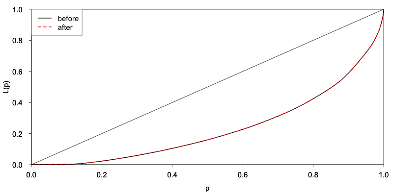
Fig. 23 Lorenz curve based on positive total expenditures values

We compare the mean monthly expenditures (MME) and mean monthly income (MMI) for rural, urban and total population. The results are shown in Table 32. We observe that the chosen levels of noise add only small distortions to the MME and slightly larger changes to the MMI.

Table 32 Mean monthly expenditure and mean monthly income per capita by rural/urban

.	before	after
MME rural	400.5	398.5
MME urban	457.3	459.9
MME total	412.6	412.6
MMI rural	397.1	402.2
MMI urban	747.6	767.8
MMI total	472.1	478.5

Table 33 shows the share of each of the components of the expenditure variables before and after anonymization.

Table 33 Shares of expenditures components

.	TFOODEXP	TALCHEXP	TCLTHEXP	THOUSEXP	TFURNEXP	THLTHEXP
before	0.58	0.01	0.03	0.09	0.02	0.03
after	0.59	0.01	0.03	0.09	0.02	0.03
.	TTRANSEXP	TCOMMEXP	TRECEXP	TEDUEXP	TRESHOTEXP	TMISCEXP
before	0.04	0.02	0.00	0.08	0.03	0.05
after	0.04	0.02	0.00	0.08	0.03	0.05

Anonymization for the creation of a SUF will inevitably lead to some degree of utility loss. It is important to describe this loss in the external report, so that users are aware of the changes in the data. This is described in Step 11 and presented in Appendix C. Appendix C also shows summary statistics and tabulations of the household level variables before and after anonymization.

Merging the household- and individual-level variables

The next step is to merge the treated household variables with the untreated individual variables for the anonymization of the individual level variables. Listing 21 shows the steps to merge these files. This also includes the selection of variables used in the anonymization of the individual-level variables. We create the sdcMicro object for the anonymization of the individual variables in the same way as for the household variable in Listing 9. Subsequently, we repeat Steps 6-10 for the individual-level variables.

Listing 21 Merging the files with household and individual-level variables and creating an sdcMicro object for the anonymization of the individual-level variables

### Select variables (individual level)
# Key variables (individual level)
selectedKeyVarsIND = c('GENDER', 'REL', 'MARITAL', 'AGEYRS',
                       'EDUCY', 'ATSCHOOL', 'INDUSTRY1') # list of selected key variables

# Sample weight (WGTHH, individual weight)
selectedWeightVarIND = c('WGTHH')

# Household ID
selectedHouseholdID = c('IDH')

# No strata

# Recombining anonymized HH datasets and individual level variables
indVars <- c("IDH", "IDP", selectedKeyVarsIND, "WGTHH") # HID and all non HH variables
fileInd <- file[indVars] # subset of file without HHVars

HHmanip <- extractManipData(sdcHH) # manipulated variables HH
HHmanip <- HHmanip[HHmanip[,'IDH'] != 1782,]

fileCombined <- merge(HHmanip, fileInd, by.x= c('IDH'))

fileCombined <- fileCombined[order(fileCombined[,'IDH'],
fileCombined[,'IDP']),]

dim(fileCombined)

# SDC objects with all variables and treated HH vars for
# anonymization of individual level variables
sdcCombined <- createSdcObj(dat = fileCombined, keyVars = selectedKeyVarsIND,
                            weightVar = selectedWeightVarIND, hhId = selectedHouseholdID)

Step 6b: Assessing disclosure risk (individual level)

All key variables at the individual level are categorical. Therefore, we can use k-anonymity and the individual and global risk measures (see the Sections Individual risk and Global risk). The hierarchical risk is now of interest, given the household structure in the dataset fileCombined, which includes both household- and individual-level variables. The number of individuals (absolute and relative) that violate k-anonymity at the levels 2, 3 and 5 are shown in Table 34.

Note

k-anonymity does not consider the household structure and therefore underestimates the risk. Therefore, we are more interested in the individual and global hierarchical risk measures.

Table 34 k-anonymity violations

k-anonymity	Number HH violating	Percentage
2	998	9.91%
3	1,384	13.75%
5	2,194	21.79%

The global risk measures can be found using R as illustrated in Listing 22. The global risk is 0.24%, which corresponds to 24 expected re-identifications. Accounting for the hierarchical structure, this rises to 1.26%, or 127 expected re-identifications. The global risk measures are low compared to the number of \(k\)-anonymity violators due to the low sampling weights. The high number of \(k\)-anonymity violators is mainly due to the very detailed age variable. The risk measures are based only on the individual level variables, since we assume that the individual and household level variables are be used simultaneously by an intruder. If we would consider an intruder scenario where these variables are used simultaneously by an intruder to re-identify individuals, the household level variables should also be taken into account here. This would results in a high number of key variables.

Listing 22 Global risk of the individual-level variables

print(sdcCombined, 'risk')
## Risk measures:
##
## Number of observations with higher risk than the main part of the data: 0
## Expected number of re-identifications: 23.98 (0.24 %)
##
## Information on hierarchical risk:
## Expected number of re-identifications: 127.12 (1.26 %)

Step 7b: Assessing utility (individual level)

We evaluate the utility measures selected in Step 5 besides some general utility measures. The values computed from the raw data are presented in step 10b to allow for direct comparison with the values computed from the anonymized data.

Step 8b: Choice and application of SDC methods (individual level)

We use the same approach for the anonymization of the individual-level categorical key variables as for the household level categorical variables described earlier: first use global recoding to limit the necessary number of suppressions, then apply local suppressions and finally, if necessary, use of perturbative methods.

The variable AGEYRS (i.e., age in years) has many different values (age in months for children 0 – 1 years and age in years for individuals over 1 year). This level of detail leads to a high level of re-identification risk, given external datasets with exact age as well as knowledge of the exact age of close relatives. We have to reduce the level of detail in the age variables by recoding the age values (see the Section Recoding ). First, we recode the values from 15 to 65 in ten-year intervals. Since some indicators related to education are computed from the survey dataset, our first approach is not to recode the age range 0 – 15 years. For children under the age of 1 year, we reduce the level of detail and recode these to 0 years. These recodes are shown in Listing 23. We also top-code age at the age of 65 years. This protects individuals with high (rare) age values.

Listing 23 Recoding age in 10-year intervals in the range 15 – 65 and top code age over 65 years

# Recoding age and top coding age (top code 65), below that 10 year age
# groups, children aged under 1 are recoded 0 (previously in months)

sdcCombined@manipKeyVars$AGEYRS[sdcCombined@manipKeyVars$AGEYRS >= 0 &
sdcCombined@manipKeyVars$AGEYRS < 1] <- 0

sdcCombined@manipKeyVars$AGEYRS[sdcCombined@manipKeyVars$AGEYRS >= 15 &
sdcCombined@manipKeyVars$AGEYRS < 25] <- 20

...

sdcCombined@manipKeyVars$AGEYRS[sdcCombined@manipKeyVars$AGEYRS >= 55 &
sdcCombined@manipKeyVars$AGEYRS < 66] <- 60

# topBotCoding also recalculates risk based on manual recoding above
sdcCombined <- **topBotCoding(obj = sdcCombined, value = 65,
replacement = 65, kind = 'top', column = 'AGEYRS')

table(sdcCombined@manipKeyVars$AGEYRS) # check results
##    0    1    2    3    4    5    6    7    8    9   10   11   12   13   14
##  311  367  340  332  260  334  344  297  344  281  336  297  326  299  263
##   20   30   40   50   60   65
## 1847 1220  889  554  314  325

These recodes already reduce the risk to 531 individuals violating 3-anonymity. We could recode the values of age in the lower range according to the age categories users require (e.g., 8 – 11 for education). There are many different categories for different indicators, however, including education indicators. This would reduce the utility of the data for some users. Therefore, we decide to look first at the number of suppressions needed in local suppression after this limited recoding. If the number of suppressions is too high, we can go back and recode age in the range 1 – 14 years.

In Listing 24 we demonstrate how one might experiment with local suppression to find the best option. We use local suppression to achieve 3-anonymity (see the Section Local suppression . On the first attempt, we do not specify any importance vector; this leads to many suppressions in the variable AGEYRS (see Table 35 below, first row), however. This is undesirable from a utility point of view. Therefore, we decide to specify an importance vector to prevent suppressions in the variable AGEYRS. Suppressing the variable GENDER is also undesirable from the utility point of view. The variable GENDER is a type of variable that should not have suppressions. We set GENDER as variable with the second highest importance. After specifying the importance vector to prevent suppressions of the age variable, there are no age suppressions (see Table 35, second row). The total number of suppressions in the other variables increased, however, from 253 to 323 because of the importance vector. This is to be expected because the algorithm without the importance vector minimizes the total number of suppressions by first suppressing values in variables with many categories – in this case, age and gender. Specifying an importance vector prevents reaching this optimality and hence leads to a higher total number of suppressions. There is a trade-off between which variables are suppressed and the total number of suppressions. After specifying an importance vector, the variable REL has many suppressions (see Table 35, second row). We choose this second option.

Listing 24 Experimenting with different options in local suppression

# Copy of sdcMicro object to later undo steps
sdcCopy <- sdcCombined

# Importance vectors for local suppression (depending on utility measures)
impVec1 <- NULL # for optimal suppression
impVec2 <- rep(length(selectedKeyVarsIND), length(selectedKeyVarsIND))
impVec2[match('AGEYRS', selectedKeyVarsIND)] <- 1 # AGEYRS
impVec2[match('GENDER', selectedKeyVarsIND)] <- 2 # GENDER

# Local suppression without importance vector
sdcCombined <- localSuppression(sdcCombined, k = 2, importance = impVec1)

# Number of suppressions per variable
print(sdcCombined, "ls")

## Local Suppression:
##       KeyVar | Suppressions (#) | Suppressions (%)
##       GENDER |                0 |            0.000
##          REL |               34 |            0.338
##      MARITAL |                0 |            0.000
##       AGEYRS |              195 |            1.937
##        EDUCY |                0 |            0.000
##  EDYRSCURRAT |                3 |            0.030
##     ATSCHOOL |                0 |            0.000
##    INDUSTRY1 |               21 |            0.209

# Number of suppressions per variable for each value of AGEYRS
table(sdcCopy@manipKeyVars$AGEYRS) - table(sdcCombined@manipKeyVars$AGEYRS)

##  0  1  2  3  4  5  6  7  8  9 10 11 12 13 14 20 30 40 50 60 65
##  0  0  0  0  0  0  2  0  2  1  0  1  4  1  5 25 53 37 36 15 13

# Undo local suppression
sdcCombined <- undolast(sdcCombined)

# Local suppression with importance vector on AGEYRS and GENDER
sdcCombined <- localSuppression(sdcCombined, k = 2, importance = impVec2)

# Number of suppressions per variable
print(sdcCombined, "ls")
## Local Suppression:
##       KeyVar | Suppressions (#) | Suppressions (%)
##       GENDER |                0 |            0.000
##          REL |              323 |            3.208
##      MARITAL |                0 |            0.000
##       AGEYRS |                0 |            0.000
##        EDUCY |                0 |            0.000
##  EDYRSCURRAT |                0 |            0.000
##     ATSCHOOL |                0 |            0.000
##    INDUSTRY1 |                0 |            0.000

# Number of suppressions for each value of the variable AGEYRS
table(sdcCopy@manipKeyVars$AGEYRS) - table(sdcCombined@manipKeyVars$AGEYRS)
##  0  1  2  3  4  5  6  7  8  9 10 11 12 13 14 20 30 40 50 60 65
##  0  0  0  0  0  0  0  0  0  0  0  0  0  0  0  0  0  0  0  0  0

Table 35 Number of suppressions by variable for different variations of local suppression

Local suppression options	GENDER	REL	MARITAL	AGEYRS	EDUCY	EDYRSCURATT	ATSCHOOL	INDUSTRY1
k = 2, no imp	0	34	0	195	0	3	0	21
k = 2, imp on AGEYRS	0	323	0	0	0	0	0	0

Step 9b: Re-measure risk (individual level)

We re-evaluate the risk measures selected in Step 6b. Table 36 shows that local suppression, not surprisingly, has reduced the number of individuals violating 2-anonymity to 0.

Table 36 k-anonymity violations

k-anonymity	Number HH violating	Percentage
2	0	0.00 %
3	197	1.96 %
5	518	5.15 %

The hierarchical global risk was reduced to 0.11%, which corresponds to 11.3 expected re-identifications. The highest individual hierarchical re-identification risk is 1.21%. These risk levels would seem acceptable for a SUF.

Step 10b: Re-measure utility (individual level)

We selected two utility measures for the individual variables: primary and secondary education enrollment, both also by gender. These two measures are sensitive to changes in the variables gender (GENDER), age (AGEYRS) and education (EDUCY and EDYRSATCURR), and therefore give a good overview of the impact of the anonymization. As shown in Table 37 the anonymization did not change the results. The results of the tabulations in Appendix C confirm these results.

Table 37 Net enrollment in primary and secondary education by gender

.	Primary education			Secondary education
Before	72.6%	74.2%	70.9%	42.0%	44.8%	39.1%
After	72.6%	74.2%	70.9%	42.0%	44.8%	39.1%

Step 11: Audit and reporting

In the audit step, we check whether the data allow for reproduction of published figures from the original dataset and relationships between variables and other data characteristics are preserved in the anonymization process. In short, we check whether the dataset is valid for analytical purposes. There are no figures available that were published from the dataset and need to be reproducible from the anonymized data.

In Step 2, we explored the data characteristics and relationships between variables. These data characteristics and relationships have been mainly preserved, since we took them into account when choosing the appropriate anonymization methods. The variables TANHHEXP and INCTOTGROSSHH are the sums of the individual components, because we added noise to the components and reconstructed the aggregates by summing over the components. Initially, the income variables were all positive. This characteristic has been violated, as a result of noise addition. Since values of the variable AGEYRS were not perturbed, but only recoded and suppressed, we did not introduce unlikely combinations, such as a 60-year-old individual enrolled in primary education. Also, by separating the anonymization process into two parts, one for household-level variables and one for individual-level variables, the values of variables measured at the household level agree for all members of each household.

Furthermore, we drafted two reports, internal and external, on the anonymization of the case study dataset. The internal report includes the methods used, the risk before and after anonymization as well as the reasons for the selected methods and their parameters. The external report focuses on the changes in the data and the loss in utility. Focus here should be on the number of suppressions as well as the perturbative methods (PRAM). This is described in the previous steps.

Note

When creating a SUF, it is inevitable that there will be a loss of information and it is very important for the users to be aware of these changes and release them in a report that accompanies the data.

Appendix C provides examples of an internal and external report of the anonymization process of this dataset. Depending on the users and readers of the reports, the content may differ. The code to this case study shows how to obtain the information for the reports. Some measures are also available in the standard reports generated with the report() function. This is shown in Listing 25. The report() function will only use the data available in the sdcMicro object, which does not contain all households for sdcHH.

Listing 25 Using the report() function for internal and external reports

# Create reports with sdcMicro report() function
report(sdcHH, internal = F) # external (brief) report
report(sdcHH, internal = T) # internal (extended) report

# Create reports with sdcMicro report() function
report(sdcCombined, internal = F) # external (brief) report
report(sdcCombined, internal = T) # internal (extended) report

Step 12: Data release

The final step is the release of the anonymized dataset together with the external report. Listing 26 shows how to collect the data from the sdcMicro object with the extractManipData() function. Before releasing the file, we add an individual ID to the file (line number in household). We export the anonymized dataset in as STATA file. The Section Read functions in R presents functions for exporting files in other data formats.

Listing 26 Exporting the anonymized dataset

# Anonymized dataset
# Household variables and individual variables
# extracts all variables, not just the manipulated ones
dataAnon <- extractManipData(sdcCombined, ignoreKeyVars = F, ignorePramVars = F,
                             ignoreNumVars = F, ignoreStrataVar = F)

# Create STATA file
write.dta(dataframe = dataAnon, file= 'Case1DataAnon.dta', convert.dates=TRUE)

Case study 2 - PUF

This case study is a continuation of case study 1 in the Section Case study 1- SUF . Case study 1 produces a SUF file. In this case study we use this SUF file to produce a PUF file of the same dataset, which can be freely distributed. The structure of the SUF and PUF releases will be the same. However, the PUF will contain fewer variables and less (detailed) information than the SUF. We refer to the Section Case study 1- SUF for a description of the dataset.

Note

It is also possible to directly produce a PUF from a dataset without first creating a SUF.

As in case study 1, we show how the creation of a PUF can be achieved using the open source and free sdcMicro package and R. A ready-to-run R script for this case study and the dataset are also available to reproduce the results and allow the user to adapt the code (see http://ihsn.org/home/projects/sdc-practice). Extracts of this code are presented in this section to illustrate several steps of the anonymization process.

Note

The choices of methods and parameters in this case study are based on this particular dataset and the results and choices might be different for other datasets.

This case study follows the steps of the SDC process outlined in The SDC Process.

Step 1: Need for disclosure control

The same reasoning as in case study 1 applies: the SUF dataset produced in case study 1 contains data on individuals and households and some variables are confidential and/or sensitive. The decisions made in case study 1 are based on the disclosure scenarios for a SUF release. The anonymization applied for the SUF does not provide sufficient protection for the release as PUF and the SUF file cannot be released as PUF without further treatment. Therefore, we have to repeat the SDC process with a different set of disclosure scenarios based on the characteristics of a PUF release (see Step 4). This leads to different risk measures, lower accepted risk levels and different SDC methods.

Step 2: Data preparation and exploring data characteristics

In order to guarantee consistency between the released PUF and SUF files, which is required to prevent intruders from using the datasets together (SUF users have also access to the PUF file), we have to use the anonymized SUF file to create the PUF file (see also the Section Step 3: Type of release). In this way all information in the PUF file is also contained in the SUF, and the PUF does not provide additional information to an intruder with access to the SUF. We load the required packages to read the data (foreign package for STATA files) and load the SUF dataset into “file” as illustrated in Listing 27. We also load the original data file (raw data) as “fileOrig”. We need the raw data to undo perturbative methods used in case study 1 (see Step 8) and to compare data utility measures (see Step 5). To evaluate the utility loss in the PUF, we have to compare the information in the anonymized PUF file with the information in the raw data. For an overview of the data characteristics and a description of the variables in both files, we refer to Step 2 of Case study 1- SUF .

Listing 27 Loading required packages and datasets

# Load required packages
library(foreign)  # for read/write function for STATA
library(sdcMicro) # sdcMicro package

# Set working directory - set to the path on your machine
setwd("/Users/CaseStudy2")

# Specify file name of SUF file from case study 1
fname <- "CaseDataAnon.dta"

# Specify file name of original dataset (raw data)
fnameOrig <- "CaseA.dta"

# Read-in files
file     <- read.dta(fname, convert.factors = TRUE) # SUF file case study 1
fileOrig <- read.dta(fnameOrig, convert.factors = TRUE) # original data

We check the number of variables and number of observations of both files and the variable names of the SUF file, as shown in Listing 28. The PUF file has fewer records and fewer variables than the original data file, since we removed large households and several variables to generate the SUF file.

Listing 28 Number of individuals and variables and variable names

# Dimensions of file (observations, variables)
dim(file)
## [1] 10068    49

dim(fileOrig)
## [1] 10574    68

colnames(file) # Variable names
##  [1] "IDH"           "URBRUR"        "REGION"        "HHSIZE"
##  [5] "OWNAGLAND"     "RELIG"         "ROOF"          "TOILET"
##  [9] "WATER"         "ELECTCON"      "FUELCOOK"      "OWNMOTORCYCLE"
## [13] "CAR"           "TV"            "LIVESTOCK"     "LANDSIZEHA"
## [17] "TANHHEXP"      "TFOODEXP"      "TALCHEXP"      "TCLTHEXP"
## [21] "THOUSEXP"      "TFURNEXP"      "THLTHEXP"      "TTRANSEXP"
## [25] "TCOMMEXP"      "TRECEXP"       "TEDUEXP"       "TRESTHOTEXP"
## [29] "TMISCEXP"      "INCTOTGROSSHH" "INCRMT"        "INCWAGE"
## [33] "INCFARMBSN"    "INCNFARMBSN"   "INCRENT"       "INCFIN"
## [37] "INCPENSN"      "INCOTHER"      "WGTPOP"        "IDP"
## [41] "GENDER"        "REL"           "MARITAL"       "AGEYRS"
## [45] "EDUCY"         "EDYRSCURRAT"   "ATSCHOOL"      "INDUSTRY1"
## [49] "WGTHH"

To get an overview of the values of the variables, we use tabulations and cross-tabulations for categorical variables and summary statistics for continuous variables. To include the number of missing values (‘NA’ or other), we use the option useNA = “ifany” in the table() function. For some variables, these tabulations differ from the tabulations of the raw data, due to the anonymization of the SUF file.

In Table 38 the variables in the dataset “file” are listed along with concise descriptions of the variables, the level at which they are collected (individual level (IND) or household level (HH)), the measurement type (continuous, semi-continuous or categorical) and value ranges. Note that the dataset contains a selection of 49 variables of the 68 variable selected for the SUF release. The variables have been preselected based on their relevance for data users and some variables were removed while creating a SUF file. The numerical values for many of the categorical variables are codes that refer to values, e.g., in the variable “URBRUR”, 1 stands for ‘rural’ and 2 for ‘urban’. More information on the meanings of coded values of the categorical variables is available in the R code for this case study.

Any data cleaning, such as recoding missing value codes and removing empty variables, was already done in case study 1. The same holds for removing any direct identifiers. Direct identifiers are not released in the SUF file.

We identified the following sensitive variables in the dataset: variables related to schooling and labor force status as well as income and expenditure related variables. These variables need protection. Whether a variable is considered sensitive may depend on the release type, country and the dataset itself.

Table 38 Overview of the variables in the dataset

No.	Variable name	Description	Level	Measurement	Values
1	IDH	Household ID	HH	.	1-2,000
2	IDP	Individual ID	IND	.	1-13
3	REGION	Region	HH	categorical	1-6
4	URBRUR	Area of residence	HH	categorical	1, 2
5	WGTHH	Individual weighting coefficient	HH	weight	31.2-8495.7
6	WGTPOP	Population weighting coefficient	IND	weight	45.8-93452.2
7	HHSIZE	Household size	HH	semi-continuous	1-33
8	GENDER	Gender	IND	categorical	0, 1
9	REL	Relationship to household head	IND	categorical	1-9
10	MARITAL	Marital status	IND	categorical	1-6
11	AGEYRS	Age in completed years	IND	semi-continuous	0-65
12	RELIG	Religion of household head	HH	categorical	1, 5-7, 9
13	ATSCHOOL	Currently enrolled in school	IND	categorical	0, 1
14	EDUCY	Highest level of education attended	IND	categorical	1-6
15	EDYRSCUR AT	Years of education for currently enrolled	IND	semi-continuous	1-18
16	INDUSTRY	Industry classification (1-digit)	IND	categorical	1-10
17	ROOF	Main material used for roof	IND	categorical	1-5, 9
18	TOILET	Main toilet facility	HH	categorical	1-4, 9
19	ELECTCON	Electricity	HH	categorical	0-3
20	FUELCOOK	Main cooking fuel	HH	categorical	1-5, 9
21	WATER	Main source of water	HH	categorical	1-9
22	OWNAGLAN	Ownership of agricultural land	HH	categorical	1-3
23	LANDSIZE	Land size owned by household (ha) (agric and non agric)	HH	continuous	0-40
24	OWNMOTORYCLE	Ownership of motorcycle	HH	categorical	0, 1
25	CAR	Ownership of car	HH	categorical	0, 1
26	TV	Ownership of television	HH	categorical	0, 1
27	LIVESTOC	Number of large-sized livestock owned	HH	semi-continuous	0-25
28	INCRMT	Income – Remittances	HH	continuous
29	INCWAGE	Income - Wages and salaries	HH	continuous
30	INCFARMBSN	Income - Gross income from household farm businesses	HH	continuous
31	INCNFARMBSN	Income - Gross income from household nonfarm businesses	HH	continuous
32	INCRENT	Income - Rent	HH	continuous
33	INCFIN	Income - Financial	HH	continuous
34	INCPENSN	Income - Pensions/social assistance	HH	continuous
35	INCOTHER	Income - Other	HH	continuous
36	INCTOTGROSHH	Income - Total	HH	continuous
37	FARMEMP
38	TFOODEXP	Total expenditure on food	HH	continuous
39	TALCHEXP	Total expenditure on alcoholic beverages, tobacco and narcotics	HH	continuous
40	TCLTHEXP	Total expenditure on clothing	HH	continuous
41	THOUSEXP	Total expenditure on housing	HH	continuous
42	TFURNEXP	Total expenditure on furnishing	HH	continuous
43	THLTHEXP	Total expenditure on health	HH	continuous
43	TTRANSEXP	Total expenditure on transport	HH	continuous
44	TCOMMEXP	Total expenditure on communication	HH	continuous
45	TRECEXP	Total expenditure on recreation	HH	continuous
46	TEDUEXP	Total expenditure on education	HH	continuous
47	TRESHOTEXP	Total expenditure on restaurants and hotels	HH	continuous
48	TMISCEXP	Total expenditure on miscellaneous spending	HH	continuous
49	TANHHEXP	Total annual nominal household expenditures	HH	continuous

It is always important to ensure that the relationships between variables in the data are preserved during the anonymization process and to explore and take note of these relationships before beginning the anonymization. At the end of the anonymization process before the release of the data, an audit should be conducted, using these initial results, to check that these relationships are maintained in the anonymized dataset (see Step 11).

In our dataset, we identify several relationships between variables that need to be preserved during the anonymization process. The variables “TANHHEXP” and “INCTOTGROSSHH” represent the total annual nominal household expenditure and the total gross annual household income, respectively, and these variables are aggregations of existing income and expenditure components in the dataset.

The variables related to education are available only for individuals in the appropriate age groups and missing for other individuals. In addition, the household-level variables (cf. fourth column of Table 38) have the same values for all members in any particular household. The value of household size corresponds to the actual number of individuals belonging to that household in the dataset. As we proceed, we have to take care that these relationships and structures are preserved in the anonymization process.

We assume that the data are collected in a survey that uses simple sampling of households. The data contains two weight coefficients: “WGTHH” and “WGTPOP”. The relationship between the weights is \(WGTPOP = WGTHH * HHSIZE\). “WGTPOP” is the sampling weight for the households and “WGTHH” is the sampling weight for the individuals to be used for disclosure risk calculations. “WGTHH” is used for computing individual-level indicators (such as education) and “WGTPOP” is used for population level indicators (such as income indicators). There are no strata variables available in the data. We will use “WGTPOP” for the anonymization of the household variables and “WGTHH” for the anonymization of the individual-level variables.

Step 3: Type of release

In this case study, we assume that the file will be released as a PUF, which will be freely available to anyone interested in the data (see the Section Conditions for PUFs for the conditions and more information on the release of PUFs). The PUF release is intended for users with lower information requirements (e.g., students) and researchers interested in the structure of the data and willing to do preliminary research. The PUF file can give an idea to the researcher whether it is worthwhile for their research to apply for access to the SUF file. Researchers willing to do more in-depth research will most likely apply for SUF access. Generally, users of a PUF file are not restricted by an agreement that prevents them from using the data to re-identify individuals and hence the accepted risk level is much lower than in the case of the SUF and the set of released variables is limited.

Step 4: Intruder scenarios and choice of key variables

Next, based on the release type, we reformulate the intruder scenarios for the PUF release. This leads to the selection of a set of quasi-identifiers. Since this case study is based on a demo dataset, we do not have a real context and we cannot define exact disclosure scenarios. Therefore, we make hypothetical assumptions on possible disclosure scenarios. We consider two types of disclosure scenarios: 1) matching with other publically available datasets and 2) spontaneous recognition. Since the dataset will be distributed as PUF, there are de facto no restrictions on the use of the dataset by intruders.

For the sake of illustration, we assume that population registers are available with the demographic variables gender, age, place of residence (region, urban/rural), religion and other variables such as marital status and variables relating to education and professional status that are also present in our dataset. In addition, we assume that there is a publically available cadastral register on land ownership. Based on this analysis of available data sources, we have selected in case study 1 the variables “REGION”, “URBRUR”, “HHSIZE”, “OWNAGLAND”, “RELIG”, “GENDER”, “REL” (relationship to household head), “MARITAL” (marital status), “AGEYRS”, “INDUSTRY1” and two variables relating to school attendance as categorical quasi-identifiers, the expenditure and income variables as well as LANDSIZEHA as continuous quasi-identifiers. According to our assessment, these variables might enable an intruder to re-identify an individual or household in the dataset by matching with other available datasets. The key variables for PUF release generally coincide with the key variables for the SUF release. Possibly, more variables could be added, since the user has more possibilities to match the data extensively and is not bound by any contract, as is in the case of the SUF file. Equally, some key variables in the SUF file may not be released in the PUF file and, as a consequence, these variables are removed from the list of key variables.

Upon further consideration, this initial set of identifying variables is too large for a PUF release, as the number of possible combinations (keys) is very high and hence many respondents could be identified based on these variables. Therefore, we decide to limit the set of key variables, by excluding variables from the dataset for PUF release. The choice of variables to be removed is led by the needs of the intended PUF users. Assuming the typical users are mainly interested in aggregate income and expenditure data, we can therefore remove from the initial set of key variables “OWNAGLAND”, “RELIG” and “LANDSIZEHA” at the household level and “EDYRSCURRAT” and “ATSCHOOL” at the individual level.

Note

These variables will not be released in the PUF file.

We also remove the income and expenditure components from the list of key variables, since we reduce their information content by building proportions (see Step 8a). The list of the remaining key variables is presented in Table 39.

Table 39 Overview of selected key variables for PUF file

Variable name	Variable description	Measurement level
REGION	region	Household, categorical
URBRUR	area of residence	Household, categorical
HHSIZE	household size	Household, categorical
TANHHEXP	total expenditure	Household, continuous
INCTOTGROSSHH	total income	Household, continuous
GENDER	gender	Individual, categorical
REL	relationship to household head	Individual, categorical
MARITAL	marital status	Individual, categorical
AGEYRS	age in completed years	Individual, semi-continuous/categorical
EDUCY	highest level of education completed	Individual, categorical
INDUSTRY1	industry classification	Individual, categorical

The decision to release the dataset as a PUF means the level of anonymization will be relatively high and consequently, the variables are less detailed (e.g., after recoding) and a scenario of spontaneous recognition is less likely. Nevertheless, we should check for rare combinations or unusual patterns in the variables. Variables that may lead to spontaneous recognition in our sample are amongst others “HHSIZE” (household size) as well as “INCTOTGROSSHH” (aggregate income) and “TANHHEXP” (total expenditure). Large households and households with high income are easily identifiable, especially when combined with other identifying variables such as a geographical identifier (“REGION”). There might be only one or a few households/individuals in a certain region with a high income, such as the local doctor. Variables that are easily observable and known by neighbors such as “ROOF”, “TOILET”, “WATER”, “ELECTCON”, “FUELCOOK”, “OWNMOTORCYCLE”, “CAR”, “TV” and “LIVESTOCK” may also need protection depending on what stands out in the community, since a user might be able to identify persons (s)he knows. This is called the nosy-neighbor scenario.

Step 5: Data key uses and selection of utility measures

A PUF file contains less information and the file is generally used by students as a teaching file, by researchers to get an idea about the data structure, and for simple analyses. The users have generally lower requirements than for a SUF file and the results of analysis may be less precise. The researcher interested in a more detailed dataset, would have to apply for access to the SUF file. Therefore, we select more aggregate utility measures for the PUF file that reflect the intended use of a PUF file. Data intensive measures, such as the Gini coefficient, cannot be computed from the PUF file. Besides the standard utility measures, such as tabulations, we evaluate the decile dispersion ratio and a regression with the income deciles as regressand.

To measure the information loss, we should compare the initial data file before any anonymization (including the anonymization for the SUF) with the file after the anonymization for the PUF. Comparing the files directly before and after the PUF anonymization would underestimate the information loss, as this would omit the information loss due to SUF anonymization. Therefore, in Step 2, we also loaded the raw dataset.

Hierarchical (household) structure

As noted in case study 1, the data has a household structure. For the SUF release, we protected large households by removing these from the dataset. Since some variables are measured on the household level and thus have identical values for each household member, the values of the household variables should be treated in the same way for each household member (see the Section Anonymization of the quasi-identifier household size ). Therefore, we first anonymize only the household variables. After this, we merge them with the individual-level variables and then anonymize the individual-level and household-level variables jointly.

Since the data has a hierarchical structure, Steps 6 through 10 are repeated twice: Steps 6a through 10a are for the household-level variables and Steps 6b through 10b for the combined dataset. In this way, we ensure that household-level variable values remain consistent across household members for each household and the household structure cannot be used to re-identify individuals. This is further explained in the Sections Levels of risk and Household structure.

Before continuing to Step 6a, we select the categorical key variables, continuous key variables and any variables selected for use in PRAM routines, as well as household-level sampling weights in R. We also collect the variable names of the variables that will not be released. The PRAM variables are variables select for the PRAM routine, which we discuss further in Step 8a. We extract these selected household variables from the SUF dataset and save them as “fileHH”. The choice of PRAM variables is further explained in Step 8a. Listing 29 illustrates how these steps are done in R (see also the Section Household structure).

Listing 29 Selecting the variables for the household-level anonymization

# Categorical key variables at household level
selectedKeyVarsHH <- c('URBRUR', 'REGION', 'HHSIZE')

# Continuous key variables
numVarsHH <- c('TANHHEXP', 'INCTOTGROSSHH')

# PRAM variables
pramVarsHH <- c('ROOF', 'TOILET', 'WATER', 'ELECTCON',
                'FUELCOOK', 'OWNMOTORCYCLE', 'CAR', 'TV', 'LIVESTOCK')

# Household weight
weightVarHH <- c('WGTPOP')

# Variables not suitable for release in PUF (HH level)
varsNotToBeReleasedHH <- c("OWNAGLAND", "RELIG", "LANDSIZEHA")

# Vector with names of all HH level variables
HHVars <- c('IDH', selectedKeyVarsHH, pramVarsHH, numVarsHH, weightVarHH)

# Create subset of file with only HH level variables
fileHH <- file[,HHVars]

Every household has the same number of entries as it has members (e.g., a household of three will be repeated three times in “fileHH”). Before analyzing the household-level variables, we select only one entry per household, as illustrated in Listing 30. This is further explained in the Section Household structure. In the same way we extract “fileOrigHH” from “fileOrig”. “fileOrigHH” contains all variables from the raw data, but contains every household only once. We need “fileOrigHH” in Steps 8a and 10a for undoing some perturbative methods used in the SUF file and computing utility measures from the raw data respectively.

Listing 30 Taking a subset with only households

# Remove duplicated rows based on IDH, one row per household in fileHH
fileHH <- fileHH[which(!duplicated(fileHH$IDH)),] # SUF file
fileOrigHH <- fileOrig[which(!duplicated(fileOrig$IDH)),] # original dataset

# Dimensions of fileHH
dim(fileHH)
## [1] 1970   16

dim(fileOrigHH)
## [1] 2000   68

The file “fileHH” contains 1,970 households and 16 variables. We are now ready to create our sdcMicro object with the corresponding variables we selected in Listing 28. For our case study, we will create an sdcMicro object called “sdcHH” based on the data in “fileHH”, which we will use for steps 6a – 10a (see Listing 34).

Note

When the sdcMicro object is created, the sdcMicro package automatically calculates and stores the risk measures for the data.

This leads us to Step 6a.

Listing 31 Creating a sdcMicro object for the household variables

# Create initial sdcMicro object for household level variables
sdcHH <- createSdcObj(dat = fileHH, keyVars = selectedKeyVarsHH,
                      pramVars = pramVarsHH, weightVar = weightVarHH, numVars = numVarsHH)
numHH <- length(fileHH[,1]) # number of households

Step 6a: Assessing disclosure risk (household level)

Based on the key variables selected in the disclosure scenarios, we can evaluate the risk at the household level. The PUF risk measures show a lower risk level than in the SUF file after anonymization in case study 1. The reason is that the set of key variables is smaller, since some variables will not be released in the PUF file. Removing (key) variables reduces the risk, and it is one of the most straightforward SDC methods.

As a first measure, we evaluate the number of households violating \(k\)-anonymity at the levels 2, 3 and 5. Table 40 shows the number of violating households as well as the percentage of the total number of households. Listing 32 illustrates how to find these values with sdcMicro. The print() function in sdcMicro shows only the values for thresholds 2 and 3. Values for other thresholds can be calculated manually by summing up the frequencies smaller than the \(k\)-anonymity threshold, as shown in Listing 32. The number of violators is already at a low level, due to the prior anonymization of the SUF file and the reduced set of key variables.

Table 40 Number and proportion of households violating \(k\)-anonymity

k-anonymity level	Number of HH violating	Percentage of total number of HH
2	0	0.0%
3	18	0.9%
5	92	4.7%

Listing 32 Showing number of households violating \(k\)-anonymity for levels 2, 3 and 5

# Number of observations violating k-anonymity (thresholds 2 and 3)
print(sdcHH)
## Infos on 2/3-Anonymity:
##
## Number of observations violating
##  - 2-anonymity: 0
##  - 3-anonymity: 18
##
## Percentage of observations violating
##  - 2-anonymity: 0.000 %
##  - 3-anonymity: 0.914 %
--------------------------------------------------------------------------

# Calculate sample frequencies and count number of obs. violating k(5) - anonymity
kAnon5 <- sum(sdcHH@risk$individual[,2] < 5)
kAnon5
## [1] 92

# As percentage of total
kAnon5 / numHH
## [1] 0.04670051

It is often useful to view the records of the household(s) that violate \(k\)-anonymity. This might help to find which variables cause the uniqueness of these households; this can then be used later when choosing appropriate SDC methods. Listing 32 shows how to access the values of the households violating 3 and 5-anonymity. Not surprisingly, the variable “HHSIZE” is responsible for many of the unique combinations and the origin of much of the risk. This is even the case after removing large households for the SUF release.

Listing 33 Showing records of households that violate \(k\)-anonymity

# Show values of key variable of records that violate k-anonymity
fileHH[sdcHH@risk$individual[,2] < 3, selectedKeyVarsHH] # for 3-anonymity
fileHH[sdcHH@risk$individual[,2] < 5, selectedKeyVarsHH] # for 5-anonymity

We also assess the disclosure risk of the categorical variables with the individual and global risk measures as described in the Sections Individual risk and Global risk. In “fileHH” every entry represents a household. Therefore, we use the individual non-hierarchical risk here, where the individual refers in this case to a household. “fileHH” is a subset of the complete dataset and contains only households and has, contrary to the complete dataset, no hierarchical structure. In Step 6b, we evaluate the hierarchical risk in the dataset “file”, the dataset containing both households and individuals. The individual and global risk measures automatically take into consideration the household weights, which we defined in Listing 29. In our file, the global risk measure calculated using the chosen key variables is lower than 0.01% (the smallest reported value is 0.01%, in fact the global risk is 0.0000642 %). This percentage is extremely low and corresponds to 0.13 expected re-identifications. The results are also shown in Listing 34. This low figure can be explained by the relatively small sample size of 0.25% of the total population (see case study 1). Furthermore, one should keep in mind that this risk measure is based only on the categorical quasi-identifiers at the household level.

Listing 34 Printing global risk measures

print(sdcHH, "risk")
## Risk measures:
##
## Number of observations with higher risk than the main part of the data: 0
## Expected number of re-identifications: 0.13 (0.01 %)

The global risk measure does not provide information about the spread of the individual risk measures. There might be a few households with relatively high risk, while the global (average) risk is low. Therefore we check the highest individual risk as shown in Listing 35. The individual risk of the household with the highest risk is 0.1 %, which is still very low.

Listing 35 Determining the highest individual risk

# Highest individual risk
max(sdcHH@risk$individual[, "risk"])
## [1] 0.001011633

Since the selected key variables at the household level are both categorical and numerical, the individual and global risk measures based on frequency counts do not completely reflect the disclosure risk of the entire dataset. When generating the SUF file, we concluded that recoding of continuous variables to make them all categorical would likely not satisfy the needs of the SUF users. For the PUF file it is acceptable to recode continuous variables, such as income and expenditures since PUF content is typically less detailed. In Step 8a we will recode these variables into deciles and convert them into categorical variables. Therefore, we exclude these variables from the risk calculations now We take these variables into account while remeasuring risk after anonymization.

Step 7a: Assessing utility measures (household level)

The utility of the data does not only depend on the household level variables, but on the combination of household-level and individual-level variables. Therefore, it is not useful to evaluate all the utility measures selected in Step 5 at this stage, i.e., before anonymizing the individual level variables. We restrict the initial measurement of utility to those measures that are solely based on the household variables. In our dataset, these are the measures related to income and expenditure and their distributions. The results are presented in Step 10a, together with the results after anonymization, which allow direct comparison. If after the next anonymization step it appears that the data utility has been significantly decreased by the suppression of some household level variables, we can return to this step.

Note

To analyze the utility loss, the utility measures before anonymization have to be calculated from the raw data and not from the anonymized SUF file.

Not all measures from case study 1 can be computed from the PUF file, since the information content is lower. The set of utility measures we use to evaluate the information loss in the PUF file consists of measures that need less detailed variables. This reflects the lower requirements a PUF user has on the dataset.

Step 8a: Choice and application of SDC methods (household level)

This step is divided into the anonymization of the categorical key variables and the continuous key variables, since different methods are used for both sets of variables. As already discussed in Step 4, we do not release all variables in the PUF file. At the household level “RELIG” (religion of household head), “OWNAGLAND” (land ownership) and “LANDSIZEHA” (plot size in ha) are not released in addition to the variables removed for the SUF release. For the sake of illustration, we assume that the variable “RELIG” is too sensitive and the variables “OWNAGLAND” and “LANDSIZEHA” are too identifying.

Categorical variables

We are now ready to move on to the choice of SDC methods for the categorical variables on the household level in our dataset. In the SUF file we already recoded some of the key variables and used local suppression. We only have three categorical key variables at the household level; “URBRUR”, “REGION” and “HHSIZE”. The selected categorical key variables at the household level are not suitable for recoding at this point, since the values cannot be grouped further. “URBRUR” has only two distinct categories and “REGION” has only six non-combinable regions. As noted before, the variable “HHSIZE” can be reconstructed by a headcount per household. Therefore, recoding of this variable alone does not lead to disclosure control.

Due to the relatively low risk of re-identification based on the three selected categorical household level variables, it is possible in this case to use an option like local suppression to achieve our desired level of risk. Applying local suppression when initial risk is relatively low will likely only lead to suppression of few observations and thus limit the loss of utility. If, however, the data had been measured to have a relatively high risk, then applying local suppression without previous recoding would likely result in a large number of suppressions and greater information loss. Efforts such a recoding should be taken first before suppressing values in cases where risk is initially measured as high. Recoding will reduce risk with little information loss and thus the number of suppressions, if local suppression is applied as an additional step.

We apply local suppression to reach 5-anonymity. The chosen level of five is higher than in the SUF release and is based on the release type as PUF. This leads to a total of 39 suppressions, all in the variable “HHSIZE”. As explained earlier, suppression of the value of the variable “HHSIZE” does not lead to actual suppression of this information. Therefore, we redo the local suppression, but this time we tell sdcMicro to, if possible, not suppress “HHSIZE” but one of the other variables. Alternatively, we could remove households with suppressed values of the variable “HHSIZE”, remove large households or split households.

In sdcMicro it is possible to tell the algorithm which variables are important and less important for making small changes (see also the Section Local suppression). To prevent values of the variable “HHSIZE” being suppressed, we set the importance of “HHSIZE” in the importance vectors to the highest (i.e., 1). We try two different importance vectors: the first where “REGION” is more important than “URBRUR” and the second with the importance of “REGION” and “URBRUR” swapped. Listing 36 shows how to apply local suppression and put importance on the variable “HHSIZE”.

Note

In Listing 36 we use the undolast() function in sdcMicro to go one step back after we had first applied local suppression with no importance vector.

The undolast() function restores the sdcMicro object back to the previous state (i.e., before we applied local suppression), which allows us to rerun the same command, but this time with an importance vector set. The undolast() function can only be used to go one step back.

The suppression patterns of the three different options are shown in Table 41. The importance is clearly reflected in the number of suppressions per variable. The total number of suppressions is with an importance vector higher than without an importance vector (44/73 vs. 39), but 5-anonymity is achieved in the dataset with no suppressions in the variable “HHSIZE”. This means that we do not have to remove or split households. The variable “REGION” is the type of variable that should not have any suppressions either. From that perspective we chose the third option. This leads to more suppressions, but no suppressions in “HHSIZE” and as few as possible in “REGION”.

Table 41 Number of suppressions by variable after local suppression with and without importance vector

Key variable	Number of suppressions and proportion of total
.	No importance vector	Importance HHSIZE, URBRUR, REGION	Importance HHSIZE, REGION, URBRUR
URBRUR	0 (0.0 %)	2 (0.1 %)	61 (3.1 %)
REGION	0 (0.0 %)	42 (2.1 %)	12 (0.6 %)
HHSIZE	39 (2.0 %)	0 (0.0 %)	0 (0.0 %)

Listing 36 Local suppression with and without importance vector

# Local suppression to achieve 5-anonimity
sdcHH <- localSuppression(sdcHH, k = 5, importance = NULL) # no importance vector
print(sdcHH, "ls")
## Local Suppression:
##  KeyVar | Suppressions (#) | Suppressions (%)
##  URBRUR |                0 |            0.000
##  REGION |                0 |            0.000
##  HHSIZE |               39 |            1.980
## ---------------------------------------------------------------------------

# Undo suppressions to see the effect of an importance vector
sdcHH <- undolast(sdcHH)

# Redo local suppression minimizing the number of suppressions in HHSIZE
sdcHH <- localSuppression(sdcHH, k = 5, importance = c(2, 3, 1))

print(sdcHH, "ls")
## Local Suppression:
##  KeyVar | Suppressions (#) | Suppressions (%)
##  URBRUR |                2 |            0.102
##  REGION |               42 |            2.132
##  HHSIZE |                0 |            0.000
## ---------------------------------------------------------------------------

# Undo suppressions to see the effect of a different importance vector
sdcHH <- undolast(sdcHH)

# Redo local suppression minimizing the number of suppressions in HHSIZE
sdcHH <- localSuppression*(sdcHH, k = 5, importance = c(3, 2, 1))

print(sdcHH, "ls")
## Local Suppression:
##  KeyVar | Suppressions (#) | Suppressions (%)
##  URBRUR |               61 |            3.096
##  REGION |               12 |            0.609
##  HHSIZE |                0 |            0.000
## ---------------------------------------------------------------------------

In case study 1 we applied invariant PRAM to the variables “ROOF”, “TOILET”, “WATER”, “ELECTCON”, “FUELCOOK”, “OWNMOTORCYCLE”, “CAR”, “TV” and “LIVESTOCK”, since these variables are not sensitive and were not selected as quasi-identifiers because we assumed that there are no external data sources containing this information that could be used for matching. Values can be easily observed or be known to neighbors, however, and therefore are important, together with other variables, for the nosy neighbor scenario. For the PUF release we would like to level of uncertainty by increasing the number of changes. Therefore, we redo PRAM with a different transition matrix. As discussed in the Section PRAM (Post RAndomization Method), the invariant PRAM method has the property that the univariate distributions do not change. To maintain this property, we reapply PRAM to the raw data, rather than to the already PRAMmed variables in the SUF file.

Listing 37 illustrates how to apply PRAM. We use the original values to apply PRAM and replace the values in the sdcMicro object with these values. We choose the parameter ‘pd’, the lower bound for the probability that a value is not changed, to be relatively low at 0.6. This is a lower value than the 0.8 used in the SUF file and will lead to a higher number of changes (cf. Listing 17). This is acceptable for a PUF file and introduces more uncertainty as required for a PUF release. Listing 37 also shows the number of changed records per variables. Because PRAM is a probabilistic method, we set a seed for the random number generator before applying PRAM to ensure reproducibility of the results.

Note

In some cases the choice of the seed matters. The choice of seed changes the results.

The seed should not be released, since it allows for reconstructing the original values if combined with the transition matrix. The transition matrix can be released: this allows for consistent statistical inference by correcting the statistical methods used if the researcher has knowledge about the PRAM method (at this point sdcMicro does not allow to retrieve the transition matrix).

Listing 37 Applying PRAM

# PRAM
set.seed(10987)

# Replace PRAM variables in sdcMicro object sdcHH with the original raw values
sdcHH@origData[,pramVarsHH] <- fileHH[match(fileHH$IDH, fileOrigHH$IDH), pramVarsHH]
sdcHH@manipPramVars <- fileHH[match(fileHH$IDH, fileOrigHH$IDH), pramVarsHH]

sdcHH <- pram(obj = sdcHH, pd = 0.6)
## Number of changed observations:
## - - - - - - - - - - -
## ROOF != ROOF_pram : 305 (15.48%)
## TOILET != TOILET_pram : 260 (13.2%)
## WATER != WATER_pram : 293 (14.87%)
## ELECTCON != ELECTCON_pram : 210 (10.66%)
## FUELCOOK != FUELCOOK_pram : 315 (15.99%)
## OWNMOTORCYCLE != OWNMOTORCYCLE_pram : 95 (4.82%)
## CAR != CAR_pram : 255 (12.94%)
## TV != TV_pram : 275 (13.96%)
## LIVESTOCK != LIVESTOCK_pram : 109 (5.53%)

PRAM has changed values within the variables according to the invariant transition matrices. Since we used the invariant PRAM method (see the Section PRAM (Post RAndomization Method)), the absolute univariate frequencies remain approximately unchanged. This is not the case for the multivariate frequencies. In Step 10a we compare the multivariate frequencies before and after anonymization for the PRAMmed variables.

Continuous variables

We have selected the variables “INCTOTGROSSHH” (total income) and “TANHHEXP” (total expenditure) as numerical quasi-identifiers, as discussed in Step 4. In Step 5 we identified variables having high interest for the users of our data: many users use the data for measuring inequality and expenditure patterns. The noise addition in the SUF file does not protect these variables sufficiently, especially, because outliers are not protected. Therefore, we decide to recode total income and total expenditure into deciles.

As with PRAM, we want to compute the deciles from the raw data rather than from the perturbed values in the SUF file. We compute the deciles directly from the raw data and overwrite these values in the sdcMicro object. Subsequently, we compute the mean of each decile from the raw data and replace the values for total income and total expenditures with the mean of the respective decile. In this way the mean of both variables does not change. This approach can be interpreted as univariate microaggregation with very large groups (group size n/10) with the mean as replacement value (see the Section Microaggregation).

The information in the income and expenditure variables by component is too sensitive to release as PUF, and, summing those variables would allow an intruder to reconstruct the totals. PUF users might however be interested in the shares. Therefore, we decide to keep the income and expenditure components as proportions of the raw totals, rounded to two digits. The anonymization of the income and expenditure variables is shown in Listing 38.

Listing 38 Anonymization of income and expenditure variables

# Create bands (deciles) for income and expenditure variables
(aggregates) based on the original data
decExp <- as.numeric(cut(fileOrigHH[match(fileHH$IDH, fileOrigHH$IDH), "TANHHEXP"],
                         quantile(fileOrigHH[match(fileHH$IDH, fileOrigHH$IDH), "TANHHEXP"],
                                  (0:10)/10, na.rm = T),
                         include.lowest = TRUE, labels = c(1, 2, 3, 4, 5, 6, 7, 8, 9, 10)))
 decInc <- as.numeric(cut(fileOrigHH[match(fileHH$IDH, fileOrigHH$IDH), "INCTOTGROSSHH"],
                          quantile(fileOrigHH[match(fileHH$IDH, fileOrigHH$IDH), "INCTOTGROSSHH"],
                                   (0:10)/10, na.rm = T),
                          include.lowest = TRUE, labels  = c(1, 2, 3, 4, 5, 6, 7, 8, 9, 10)))

# Mean values of deciles
decExpMean <- round(sapply(split(fileOrigHH[match(fileHH$IDH, fileOrigHH$IDH), "TANHHEXP"],
                                 decExp), mean))
decIncMean <- round(sapply(split(fileOrigHH[match(fileHH$IDH, fileOrigHH$IDH), "INCTOTGROSSHH"],
                                decInc), mean))

# Replace with mean value of decile
sdcHH@manipNumVars$TANHHEXP <- decExpMean[match(decExp,names(decExpMean))]
sdcHH@manipNumVars$INCTOTGROSSHH <- decIncMean[\ match(decInc, names(decIncMean))]

# Recalculate risks after manually changing values in sdcMicro object calcRisks(sdcHH)
calcRisks(sdcHH)

# Extract data from sdcHH
HHmanip <- extractManipData(sdcHH) # manipulated variables HH

# Keep components of expenditure and income as share of total,
# use original data since previous data was perturbed
compExp <- c('TFOODEXP', 'TALCHEXP', 'TCLTHEXP', 'THOUSEXP',
             'TFURNEXP', 'THLTHEXP', 'TTRANSEXP', 'TCOMMEXP',
             'TRECEXP', 'TEDUEXP', 'TRESTHOTEXP', 'TMISCEXP')
compInc <- c('INCRMT',  'INCWAGE', 'INCFARMBSN', 'INCNFARMBSN',
             'INCRENT', 'INCFIN',  'INCPENSN',   'INCOTHER')
HHmanip <- cbind(HHmanip, round(fileOrigHH[match(fileHH$IDH, fileOrigHH$IDH), compExp] /
                                fileOrigHH[match(fileHH$IDH, fileOrigHH$IDH),
                                           "TANHHEXP"], 2))
HHmanip <- cbind(HHmanip, round(fileOrigHH[match(fileHH$IDH, fileOrigHH$IDH), compInc] /
                                fileOrigHH[match(fileHH$IDH, fileOrigHH$IDH),
                                           "INCTOTGROSSHH"], 2))

Step 9a: Re-measure risk (household level)

For the categorical variables, we conclude that we have achieved 5-anonymity in the data with local suppression. 5-anonymity also implies 2- and 3-anonymity. The global risk stayed close to zero (as the expected number of re-identifications), which is very low. Therefore, we conclude that based on the categorical variables, the data has been sufficiently anonymized. One should keep in mind that the anonymization methods applied are complementing the ones used for the SUF.

Note

The methods selected methods in this case study alone would not be sufficient to protect the data set for a PUF release.

We have reduced the risk of spontaneous recognition of households, by removing the variable “LANDSIZEHA” and PRAMming the variables identified to be important in the nosy neighbor scenario. An intruder cannot know with certainty whether a household that (s)he recognizes in the data is the correct household, due to the noise in these variables.

These measures refer only to the categorical variables. To evaluate the risk of the continuous variables we could use an interval measure or closest neighbor algorithm. These risk measures are discussed in the Section Risk measures for continuous variables. We chose to use an interval measure, since exact value matching is not our largest concern based on the assumed scenarios and external data sources. Instead, datasets with similar values but not the exact same values could be used for matching. Here the main concern is that the values are sufficiently far from the original values, which is measured with an interval measure.

Listing 39 shows how to evaluate the interval measure for the variables “INCTOTGROSSHH” and “TANHHEXP” (total income and expenditure). The different values of the parameter \(k\) in the function dRisk() define the size of the interval around the original value as a function of the standard deviation, as explained in the Section Interval measure . The larger \(k\), the larger the intervals, the higher the probability that a perturbed value is in the interval around the original value and the higher the risk measure. The results are satisfactory, especially when keeping in mind that there are only 10 distinct values in the dataset (the means of each of the deciles). All outliers have been recoded. Looking at the proportions of the components, we do not detect any outliers (households with an unusual high or low spending pattern in one component).

Listing 39 Measuring risk of re-identification of continuous variables

# Risk evaluation continuous variables
dRisk(sdcHH@origData[,c("TANHHEXP", "INCTOTGROSSHH")],
      xm = sdcHH@manipNumVars[,c("TANHHEXP", "INCTOTGROSSHH")], k = 0.01)
## [1] 0.4619289

dRisk(sdcHH@origData[,c("TANHHEXP", "INCTOTGROSSHH")],
      xm = sdcHH@manipNumVars[,c("TANHHEXP", "INCTOTGROSSHH")], k = 0.02)
## [1] 0.642132

dRisk(sdcHH@origData[,c("TANHHEXP", "INCTOTGROSSHH")],
      xm = sdcHH@manipNumVars[,c("TANHHEXP", "INCTOTGROSSHH")], k = 0.05)
## [1] 0.8258883

Step 10a Re-measure utility (household level)

The utility in the data has decreased compared to the raw data, mainly because variables were completely removed. Many of the utility measures used in case study 1 are not applicable to the PUF file. However, by replacing the deciles with their means, we can still use the income and expenditure variables for arithmetic operations. Also the shares of the income and expenditure components can still be used, since they are based on the raw data.

We select two additional utility measures: the decile dispersion ratio and the share of total consumption by the poorest decile. The decile dispersion ratio is the ratio of the average income of the top decile and the average income of the bottom decile. Listing 40 shows how to compute these from the raw data and the household variables after anonymization. Table 42 presents the estimated values. The differences are small and mainly due to the removed households.

Table 42 Comparison of utility measures

.	Raw data	PUF file
Decile dispersion ratio	24.12	23.54
Share of consumption by the poorest decile	0.0034	0.0035

Listing 40 Computation of decile dispersion ratio and share of total consumption by the poorest decile

# Decile dispersion ratio
# raw data
mean(tail(sort(fileOrigHH$INCTOTGROSSHH), n = 200)) /
  mean(head(sort(fileOrigHH$INCTOTGROSSHH), n = 200))
## [1] 24.12152

mean(tail(sort(HHmanip$INCTOTGROSSHH), n = 197)) /
  mean(head(sort(HHmanip$INCTOTGROSSHH), n = 197))
## [1] 23.54179

# Share of total consumption by the poorest decile households
sum(head(sort(fileOrigHH$TANHHEXP), n = 200)) / sum(fileOrigHH$TANHHEXP)
## [1] 0.003411664

sum(head(sort(HHmanip$TANHHEXP), n = 197)) / sum(HHmanip$TANHHEXP)
## [1] 0.003530457

Merging the household- and individual-level variables

The next step is to merge the treated household variables with the untreated individual variables for the anonymization of the individual level variables. Listing 41 shows the steps to merge these files. This also includes the selection of variables used in the anonymization of the individual-level variables. We create the sdcMicro object for the anonymization of the individual variables in the same way as for the household variable in Listing 31. Generally, at this stage, the household level and individual level variables should be combined and quasi-identifiers at both levels be used (see the Section Levels of risk). Unfortunately, in our dataset, this leads to long computation times. Therefore, we create two sdcMicro objects, one with all key variables (“sdcCombinedAll”) and one with only the individual level key variables (“sdcCombined”). In Step 6b we compare the risk measures for both cases and in Step 8b we discuss alternative approaches to keeping the complete set of variables. We now repeat Steps 6-10 for the individual-level variables.

Listing 41 Merging the files with household and individual-level variables and creating an sdcMicro object for the anonymization of the individual-level variables

### Select variables (individual level)
selectedKeyVarsIND = c('GENDER', 'REL', 'MARITAL',
                       'AGEYRS', 'EDUCY', 'INDUSTRY1') # list of selected key variables

# sample weight (WGTHH, individual weight)
selectedWeightVarIND = c('WGTHH')

# Household ID
selectedHouseholdID = c('IDH')

# Variables not suitable for release in PUF (IND level)
varsNotToBeReleasedIND <- c("ATSCHOOL", "EDYRSCURRAT")

# All individual level variables
INDVars <- c(selectedKeyVarsIND)

# Recombining anonymized HH data sets and individual level variables
indVars <- c("IDH", "IDP", selectedKeyVarsIND, "WGTHH") # HID and all non HH vars
fileInd <- file[indVars] # subset of file without HHVars
fileCombined <- merge(HHmanip, fileInd, by.x = c('IDH'))
fileCombined <- fileCombined[order(fileCombined[,'IDH'],  fileCombined[,'IDP']),]

dim(fileCombined)
## [1] 10068    44

# SDC objects with only IND level variables
sdcCombined <- createSdcObj(dat = fileCombined, keyVars = c(selectedKeyVarsIND),
                            weightVar = selectedWeightVarIND, hhId = selectedHouseholdID)

# SDC objects with both HH and IND level variables
sdcCombinedAll <- createSdcObj(dat = fileCombined,
                               keyVars = c(selectedKeyVarsIND, selectedKeyVarsHH ),
                               weightVar = selectedWeightVarIND, hhId = selectedHouseholdID)

Step 6b: Assessing disclosure risk (individual level)

As first measure, we evaluate the number of records violating \(k\)-anonymity at the levels 2, 3 and 5. Table 43 shows the number of violating individuals as well as the percentage of the total number of households. The second and third column refer to “sdcCombined” and the fourth and fifth column to “sdcCombinedAll”. We see that combining the individual level and household level variables leads to a large increase in the number of \(k\)-anonymity violators. The choice not to include the household level variables is pragmatically driven by the computation time and can be justified by the different type of variables on the household level and individual level. One could assume that these variables are not available in the same dataset and can therefore not simultaneously be used by an intruder to re-identify individuals.

Table 43 Number of records violating \(k\)-anonimity

.	sdcCombined		sdcCombinedAll
k-anonymity	Number of records violating	Percentage of total records	Number of records violating	Percentage of total records
2	0	0.0 %	4,048	40.2 %
3	167	1.7 %	6,107	60.7 %
5	463	4.6 %	8,292	82.4 %

The global hierarchical risk measure is 0.095%, which corresponds to approximately 10 expected re-identifications. We use here the hierarchical risk measure, since the re-identification of a single household member would lead to the re-identification of the other members of the same household too. This number is low compared to the number of \(k\)-anonymity violations, due to the high sample weights, which protect the data already to a large extent. Only 24 observations have an individual hierarchical risk higher than 1%, with a maximum of 1.17%. This is mainly because of the lower sample weights of these records. Listing 42 shows how to retrieve these measures in R.

Listing 42 Risk measures before anonymization

numIND <- length(fileCombined[,1]) # number of households

# Number of observations violating k-anonymity
print(sdcCombined)
## Infos on 2/3-Anonymity:
##
## Number of observations violating
##  - 2-anonymity: 0
##  - 3-anonymity: 167
##
## Percentage of observations violating
##  - 2-anonymity: 0.000 %
##  - 3-anonymity: 1.659 %
## ---------------------------------------------------------------------------

# Calculate sample frequencies and count number of obs. violating k(3,5) - anonymity
kAnon5 <- sum(sdcCombined@risk$individual[,2] 5)
kAnon5
## [1] 463

# As percentage of total
kAnon5 / numIND
## [1] 0.04598729

# Global risk on individual level
print(sdcCombined, 'risk')
## Risk measures:
##
## Number of observations with higher risk than the main part of the data: 0
## Expected number of re-identifications: 1.69 (0.02 %)
##
## Information on hierarchical risk:
## Expected number of re-identifications: 9.57 (0.10 %)
## ---------------------------------------------------------------------------

# Number of observation with relatively high risk
dim(fileCombined[sdcCombined@risk$individual[, "hier_risk"] > 0.01,])
## [1] 24 44

# Highest individual risk
max(sdcCombined@risk$individual[, "hier_risk"])
## [1] 0.01169091

Step 7b: Assessing utility measures (individual level)

We evaluate the utility measures as discussed in Step 5 based on the raw data (before applying any anonymization measures). The results are presented in Step 10b together with the values after anonymization to allow for direct comparison.

Step 8b: Choice and application of SDC methods (individual level)

In this step, we discuss four different techniques used for anonymization: 1) removing variables from the dataset to be released, 2) recoding of categorical variables to reduce the level of detail, 3) local suppression to achieve the required level of \(k\)-anonymity, 4) randomization of the order of the records in the file. Finally, we discuss some alternative options for treating the household structure in the dataset.

Removing variables

Additional to the variables removed from the dataset for the SUF release (see case study 1), we further reduce the number of variables in the dataset to be released. This is normal practice for PUF releases. Sensitive or identifying variables are removed, which allows to release other variables at a more detailed level. In a PUF release, the set of key variables should be limited.

In our case, we decide to remove at the individual level the variables “EDYRSCURRAT”, as this variable is too identifying (identifies whether there are school-going children in the household). We keep the variable “EDUCY” (highest level of education attended) for information on education.

Note

As an alternative to removing the variables from the dataset, one could also set all values to missing. This would allow the user to see the structure and variables contained in the SUF file.

Recoding

As noted before, PUF users require a lower level of information and therefore we can recode the key variables even further to reduce the disclosure risk. The recoding of variables in case study 1 is not sufficient for a PUF release. Therefore, we recode most of the categorical key variables from Table 39 to reduce the risk and number of necessary suppressions by local suppression. Table 44 gives an overview of the recodes made. All new categories are formed with the needs of the data user in mind. Listing 43 shows how to do this in R and also shows value labels and the univariate tabulations of these variables before and after recoding.

Table 44 Overview of recodes of categorical variables at individual level

Variable	Recoding
REL (relation to household head)	recode ‘Father/Mother’, ‘ Grandchild’, ‘Son/Daughter in law’, ‘Other relative’ to ‘Other relative’ and recode ‘Domestic help’ and ‘Non-relative’ to ‘Other’
MARITAL (marital status)	recode ‘Married monogamous’, ‘Married polygamous’, ’Common law, union coutumiere, union libre, living together’ to ‘Married/living together’ and ‘Divorced/Separated’ and ‘Widowed’ to ‘Divorced/Separated/Widowed’
AGEYRS (age in completed years)	recode values under 15 to 7 (other values have been recoded for SUF)
EDUCY (highest level of education completed)	recode ‘Completed lower secondary (or post-primary vocational education) but less than completed upper secondary’, ‘Completed upper secondary (or extended vocational/technical education)’, ‘Post secondary technical’ and ‘University and higher’ to ‘Completed lower secondary or higher’
INDUSTRY1	recode to ‘primary’, ‘secondary’ and ‘tertiary’

Listing 43 Recoding the categorical and continuous variables

# Recode REL (relation to household head)
table(sdcCombined@manipKeyVars$REL, useNA = "ifany")
##
##    1    2    3    4    5    6    7    8    9 <NA>
## 1698 1319 4933   52  765   54  817   40   63  327

# 1 - Head, 2 - Spouse, 3 - Child, 4 - Father/Mother, 5 - Grandchild, 6 - Son/Daughter in law
# 7 - Other relative, 8 - Domestic help, 9 - Non-relative
sdcCombined <- groupVars(sdcCombined, var = "REL", before = c("4", "5", "6", "7"),
                         after = c("7", "7", "7", "7")) # other relative
sdcCombined <- groupVars(sdcCombined, var = "REL", before = c("8", "9"),
                         after = c("9", "9")) # other

table(sdcCombined@manipKeyVars$REL, useNA = "ifany")
##
##    1    2    3    7    9 <NA>
## 1698 1319 4933 1688  103  327

# Recode MARITAL (marital status)
table(sdcCombined@manipKeyVars$MARITAL, useNA = "ifany")

##
##    1    2    3    4    5    6 <NA>
## 3542 2141  415  295  330  329 3016

# 1 - Never married, 2 - Married monogamous, 3 - Married polygamous,
# 4 - Common law, union coutumiere, union libre, living together, 5 - Divorced/Separated,
# 6 - Widowed
sdcCombined <- groupVars(sdcCombined, var = "MARITAL", before = c("2", "3", "4"),
                         after = c("2", "2", "2")) # married/living together
sdcCombined <- groupVars(sdcCombined, var = "MARITAL", before = c("5", "6"),
                         after = c("9", "9")) # divorced/seperated/widowed*

table(sdcCombined@manipKeyVars$MARITAL, useNA = "ifany")
##
##    1    2    9 <NA>
## 3542 2851  659 3016

# Recode AGEYRS (0-15 years)
table(sdcCombined@manipKeyVars$AGEYRS, useNA = "ifany")
##
##    0    1    2    3    4    5    6    7    8    9   10   11   12   13   14
##  311  367  340  332  260  334  344  297  344  281  336  297  326  299  263
##   20   30   40   50   60   65 <NA>
## 1847 1220  889  554  314  325  188

sdcCombined <- groupVars(sdcCombined, var = "AGEYRS",
                         before = c("0", "1", "2", "3", "4", "5", "6", "7", "8", "9",
                                    "10", "11", "12", "13", "14"),
                         after = rep("7", 15))

table(sdcCombined@manipKeyVars$AGEYRS, useNA = "ifany")
##
##    7   20   30   40   50   60   65 <NA>
## 4731 1847 1220  889  554  314  325  188

sdcCombined <- calcRisks(sdcCombined)
# Recode EDUCY (highest level of educ compl)
table(sdcCombined@manipKeyVars$EDUCY, useNA = "ifany")
##
##    0    1    2    3    4    5    6 <NA>
## 1582 4755 1062  330  139   46  104 2050

# 0 - No education, 1 - Pre-school/ Primary not completed,
# 2 -  Completed primary, but less than completed lower secondary
# 3 - Completed lower secondary (or post-primary vocational education)
#     but less than completed upper secondary
# 4 - Completed upper secondary (or extended vocational/technical education),
# 5 - Post secondary technical
# 6 - University and higher
sdcCombined <- groupVars(sdcCombined, var = "EDUCY", before = c("3", "4", "5", "6"),
                         after = c("3", "3", "3", "3")) # completed lower secondary or higher
table(sdcCombined@manipKeyVars$EDUCY, useNA = "ifany")
##
##    0    1    2    3 <NA>
## 1582 4755 1062  619 2050

# Recode INDUSTRY1 ()
table(sdcCombined@manipKeyVars$INDUSTRY1, useNA = "ifany")
##
##    1    2    3    4    5    6    7    8    9   10 <NA>
## 5300   16  153    2   93  484   95   17   70  292 3546

# 1 - Agriculture and Fishing, 2 - Mining, 3 - Manufacturing, 4 -  Electricity and Utilities
# 5 - Construction, 6 - Commerce, 7 - Transportation, Storage and  Communication, 8 - Financial, Insurance and Real Estate
# 9 - Services: Public Administration, 10 - Other Services, 11 - Unspecified
sdcCombined <- groupVars(sdcCombined, var = "INDUSTRY1", before = c("1", "2"),
                         after = c("1", "1")) # primary
sdcCombined <- groupVars(sdcCombined, var = "INDUSTRY1", before = c("3", "4", "5"),
                         after = c("2", "2", "2")) # secondary
sdcCombined <- groupVars(sdcCombined, var = "INDUSTRY1", before = c("6", "7", "8", "9", "10"),
                         after = c("3", "3", "3", "3", "3")) # tertiary
table(sdcCombined@manipKeyVars$INDUSTRY1, useNA = "ifany")
##
##    1    2    3 <NA>
## 5316  248  958 3546

Local suppression

The recoding has reduced the risk already considerably. We use local suppression to achieve the required level of \(k\)-anonymity. Generally, the required level of \(k\)-anonymity for PUF files is 3 or 5. In this case study, we require 5-anonimity. Listing 44 shows the suppression pattern without specifying an importance vector. All suppressions are made in the variable “AGEYRS”. This is the variable with the highest number of different values, and hence considered first by the algorithm. We try different suppression patterns by specifying importance vectors, but we decide that the pattern without importance vector yields the best result. This is also the result with the lowest total number of suppressions. Less than 1 percent suppression in the age variable is acceptable. We could reduce this number by further recoding the variable “AGEYRS”.

Listing 44 Local suppression to reach 5-anonimity

# Local suppression without importance vector
sdcCombined <- localSuppression(sdcCombined, k = 5, importance = NULL)

# Number of suppressions per variable
print(sdcCombined, "ls")
## Local Suppression:
##     KeyVar | Suppressions (#) | Suppressions (%)
##     GENDER |                0 |            0.000
##        REL |                0 |            0.000
##    MARITAL |                0 |            0.000
##     AGEYRS |               91 |            0.904
##      EDUCY |                0 |            0.000
##  INDUSTRY1 |                0 |            0.000

Randomization of order of records

The records in the dataset are ordered by region and household ID. There is a certain geographical order of the households within the regions, due to the way the households IDs were assigned. Intruders could reconstruct suppressed values by using this structure. To prevent this, we randomly reorder the records within the regions. Listing 45 shows how to do this in R. We first count the number of records per region

Note

Some records have their region value suppressed, so we include the count of NAs.

Subsequently, we draw randomly household IDs, in such way that the regional division is respected. Finally, we sort the file by the new, randomized, individual ID (“IDP”). Households with suppressed values for “REGION” will be last in the reordered file. Before randomizing the order, we extract the data from the sdcMicro object “sdcCombined” as shown in Listing 45.

Listing 45 Randomizing the order of records within regions

# Randomize order of households dataAnon and recode IDH to random
number (sort file by region)
set.seed(97254)
# Sort by region
dataAnon <- dataAnon[order(dataAnon$REGION),]

# Number of households per region
hhperregion <- table(dataAnon[match(unique(dataAnon$IDH), dataAnon$IDH), "REGION"],
                     useNA = "ifany")

# Randomized IDH (household ID)
randomHHid <- c(sample(1:hhperregion[1], hhperregion[1]),
                unlist(lapply(1:(length(hhperregion)-1),
                              function(i){sample((sum(hhperregion[1:i]) + 1): sum(hhperregion[1:(i+1)]), hhperregion[(i+1)])})))

dataAnon$IDH <- rep(randomHHid, table(dataAnon$IDH)[match(unique(dataAnon$IDH),
                                      as.numeric(names(table(dataAnon$IDH))))])

# Sort by IDH (and region)
dataAnon <- dataAnon[order(dataAnon$IDH),]

Alternative options for dealing with household structure

In Step 6b we compared the disclosure risk for two cases: one with only individual level key variables and another with individual level and household level key variables combined. We decided to use only the individual level key variables to reduce the computation time and justified this choice by arguing that intruders cannot use household and individual level variables simultaneously. This might not always be the case. Therefore we explore other options to reduce the risk when taking both individual level and household level variables into account. We present two options: removing the household structure; and using options in the local suppression algorithm.

Removing household structure

We consider the risk emanating from the household structure in the dataset to be very high. We can remove the hierarchical household structure completely and treat all variables at the individual level. This entails, besides removing the household id (“IDH”), also treating variables that could be used for reconstructing households. These are, for instance, “REL” (relation to household head), “HHSIZE” (household size), and any of the household level variables, such as income and expenditure. However, not all household level variables need to be treated. For example, “REGION” is a household level variable, but the probability that this variable leads to the reconstruction of a household is low. Also, we need to reorder the records in the file, as they are sorted by households. Note that by removing the household structure, we interpret all variables as individual level variables for measuring disclosure risk. This leads to a lower need for recoding and suppression, since the hierarchical risk disappears. The reason why we did not opt for this approach is the loss of utility for the user. The household structure is an important feature of the data, and should be kept in the PUF file.

Using different options for local suppression

The long running time is mainly due to the local suppression algorithm. In the Section Local suppression we discuss options to reduce the running time of the local suppression in case of many key variables. The all-\(m\) approach reduces the running time by first considering subsets of the complete set of key variables. This reduces the complexity of the problem and leads to lower computation times. However, the total number of suppressions made is likely to be higher. Also, if not explicitly specified, it is not guaranteed that the required level for \(k\)-anonymity is automatically achieved on the complete set of key variables. It is therefore important to check the results.

Step 9b: Re-measure risk

We re-evaluate the risk measures selected in Step 6. Table 45 shows that local suppression, not surprisingly, has reduced the number of individuals violating 5-anonymity to 0. The global hierarchical risk was reduced to 0.02%, which corresponds to approximately 2 correct re-identifications. The highest individual hierarchical re-identification risk is 0.2%. These risk levels are acceptable for a PUF release. Furthermore, the recoding has removed any unusual combinations in the data.

Note

The risk may be underestimated by excluding the household level variables.

Table 45 k-anonymity violations

k-anonymity	Number of records violating	Percentage
2	0	0.0 %
3	0	0.0 %
5	0	0.0 %

Step 10b: Re-measure utility

We compare (cross-)tabulations before and after anonymization, which are illustrated in the R code to this case study. We note that due to the recoding in Step 8b, the detail in the variables is reduced. This reduces the number of necessary suppressions and is acceptable for a public use file.

Step 11: Audit and reporting

In the audit step, we check whether the data allow for reproduction of published figures from the original dataset and relationships between variables and other data characteristics are preserved in the anonymization process. In short, we check whether the dataset is valid for analytical purposes. There are no figures available that were published from the dataset and need to be reproducible from the anonymized data.

In Step 2, we explored the data characteristics and relationships between variables. These data characteristics and relationships have been mainly preserved, since we took them into account when choosing the appropriate anonymization methods. Since values of the variable “AGEYRS” were not perturbed, but only recoded and suppressed, we did not introduce unlikely combinations, such as a 60-year-old individual enrolled in primary education. Also, by separating the anonymization process into two parts, one for household-level variables and one for individual-level variables, the values of variables measured at the household level agree for all members of each household.

Furthermore, we drafted two reports, internal and external, on the anonymization of the case study dataset. The internal report includes the methods used, the risk before and after anonymization as well as the reasons for the selected methods and their parameters. The external report focuses on the changes in the data and the loss in utility. Focus here should be on the number of suppressions as well as the perturbative methods (PRAM). This is described in the previous steps.

Note

When creating a PUF, it is inevitable that there will be a loss of information and it is very important for the users to be aware of these changes and release them in a report that accompanies the data.

Appendix C provides examples of an internal and external report of the anonymization process of this dataset. Depending on the users and readers of the reports, the content may differ.

Note

The report() function in sdcMicro is at this point not useful, since this will only report on the SDC measures in the second case study.

However, the report should contain the entire process, including the measures applied in case study 1.

Step 12: Data release

The final step is the release of the anonymized dataset together with the external report. Listing 46 shows how to export the anonymized dataset as STATA file. The Section Read functions in R presents functions for exporting files in other data formats.

Listing 46 Exporting the anonymized PUF file

# Create STATA file
write.dta(dataframe = dataAnon, file= 'Case2DataAnon.dta', convert.dates=TRUE)

[1]	Other methods and guidance on treating datasets where household size is a quasi-identifier are discussed in the Section Anonymization of the quasi-identifier household size.

[2]	For illustrative purposes, we only show this evaluation for the expenditure variables. It can be easily copied for the income variables. The results are similar.

[3]	To compute the GINI coefficient, bootstrap to construct the confidence intervals and plot the Lorenz curve we used the R packages laeken, reldist, bootstrap and ineq.